Anomaly Detection

Anomaly detection is an important technique in data analytics that involves identifying unusual patterns or outliers in datasets. It is widely used in various applications like fraud detection, network security, and fault diagnosis. Anomalies in these datasets can indicate critical incidents such as breaches, failing components, or fraudulent transactions. To identify these anomalies, statistical, machine learning, or other data-driven methods are used to analyze data in real-time or in batches. This helps in identifying data points that deviate significantly from the expected behavior. By detecting and flagging these anomalies, organizations can proactively address potential issues, leading to improved operational efficiency and security.¹

Table of contents

1. One-Class SVM
2. Isolation Forest
3. References
4. Version History

---

One-Class SVM

The One-Class Support Vector Machine (One-Class SVM) anomaly detection algorithm is specifically designed to detect outliers or anomalies in a dataset by defining a normative region and identifying data points that deviate significantly from it. It accomplishes this by mapping the input data to a high-dimensional feature space using a kernel function. Subsequently, it seeks to find a hyperplane that maximizes the margin, separating most of the data points from the origin. The algorithm uses four types of kernel functions to achieve this transformation:²

Linear Kernel

$$ \begin{equation} K(x, x') = \langle x, x' \rangle {\qquad [1] \qquad} \end{equation} $$

This kernel represents a single dot product between two vectors. The terms $x$ and $x’$ represent vectors and are used to denote any two data points for which you are calculating the kernel. The dot product is a scalar representation of the projection of one vector onto another, indicating how much of one vector goes in the direction of another.

Polynomial Kernel

$$ \begin{equation} K(x, x') = \left( \gamma \cdot \langle x, x' \rangle + r \right)^{d} {\qquad [2] \qquad} \end{equation} $$

In the above expression \(\begin{equation} \gamma \cdot \langle x, x' \rangle \end{equation}\) involves a scalar multiplication of (a predefined scaling factor) with the dot product \(\begin{equation} \langle x, x' \rangle \end{equation}\) of the input vectors $x$ and $x’$. This kernel maps inputs into a polynomial feature space, controlled by degree $d$, where higher degrees allow for more complex decision boundaries. Coefficient $r$ adjusts the influence of higher-degree terms, and scales the input data.

RBF (Radial Basis Function) Kernel

$$ \begin{equation} K(x, x') = \exp\left( -\gamma \|x - x'\|^{2} \right) {\qquad [3] \qquad} \end{equation} $$

The RBF kernel introduces a Gaussian function of the distance between points, controlled by (here multiplies the square of the Euclidean distance), allowing it to handle varied data distributions by forming region-based boundaries.

Sigmoid Kernel

$$ \begin{equation} K(x, x') = \tanh\left( \gamma \cdot \langle x, x' \rangle + r \right) {\qquad [4] \qquad} \end{equation} $$

Similarly, to the polynomial kernel, this involves a dot product scaled by and offset by $r$, followed by the hyperbolic tangent function. This kernel uses a hyperbolic tangent function, transforming the data similar to the activation function in neural networks, which can create complex, non-linear decision boundaries.

One-Class SVM aims to maximize the margin between the data and the origin in the feature space, effectively identifying outliers in scenarios where a clear “normal” class exists. The parameters v(nu) and C determine the balance between capturing all the “normal” data points within the boundary and allowing flexibility for some outliers. This trade-off is crucial for accurate anomaly detection in applications like fraud detection and system health monitoring.

Use the One-Class SVM function by browsing in the top ribbon:

Analytics \(\rightarrow\) Anomaly Detection \(\rightarrow\) One-Class SVM

Input

The data input should consist of numerical (“normal”) instances, without any missing values. There are no inherent limitations on the number of columns or rows.

Configuration

Type of Kernel	You can choose from different types of kernels including Linear, Polynomial, RBF, and Sigmoid. Depending on the user-selection specify the parameter values in the kernel equation (Eqs. 1-4).
Generic parameters	You can also set parameters like C, Nu, Tolerance, and Cache to optimize the performance and efficiency of anomaly detection.

Output

The output sheet will have two columns: one for the prediction (expected or anomalous) and the other for the scoring.

Example

Input

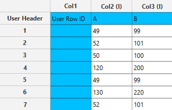
The data are inserted as shown below in the data input sheet on the left-hand side.

Configuration

1. Select Analytics \(\rightarrow\) Anomaly Detection \(\rightarrow\) One-Class SVM
2. Select the Type of kernel [1] and specify the parameter values [2] in the kernel equation. Choose appropriate values for the Generic parameters to optimize the performance and efficiency of anomaly detection [3].
3. Click on the Execute button [4] to apply the anomaly detection calculation.

Output

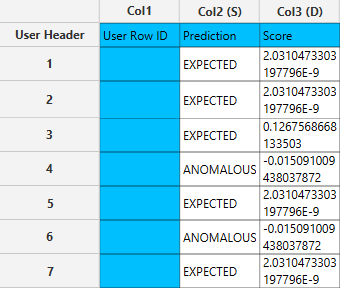
The right-hand spreadsheet tab presents two columns in the output: one for predicting whether the result is expected or anomalous, and another for the scoring.

Isolation Forest

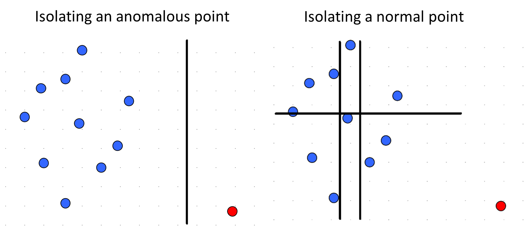
The Isolation Forest anomaly detection algorithm is designed to explicitly isolate anomalies instead of profiling normal points. To achieve this, the method leverages two properties of anomalies :

1. Anomalies are the minority consisting of fewer instances than normal points.
2. Anomalies tend to have distinct attribute values, making them easier to isolate compared to normal data points.

An Isolation Tree is a binary tree constructed by recursively selecting a random feature along with a random split value for each node and splitting data points according to them.

An Isolation Forest is an ensemble of Isolation Trees, each built using a random subsample of the training data. To compute the anomaly score for each one of the instances we measure the average path length of that instance across all Isolation Trees in the Isolation Forest and then scale this quantity using the formula:

$$ \begin{equation} s(x,n) = 2^- \frac{E(h(x))}{c(n)} \end{equation} $$

where \(E(h(x))\) is the average path length of instance x, n is the subsampling size and \(c(n)\) is an estimation of the average path length in an Isolation Tree borrowed from Binary Search Trees that is computed as follows:

$$ \begin{equation} c(n) = 2H(n-1) - \frac{2*(n-1)}{n} \end{equation} $$

where \(H(i)\) is the harmonic number, and it can be estimated as:

$$ \begin{equation} H(i) \sim ln(i) + 0.5772156649 \end{equation} $$

Instances with \(s(x)\) close to 1 are most likely anomalies, while instances with \(s(x)\) closer to zero are quite safe to be regarded as normal instances.

There are three ways to determine whether a point is considered an anomaly based on the anomaly scores produced by the algorithm:

• Contamination Factor : This method uses a contamination factor, which is the percentage of training data assumed to be anomalous. Based on this factor, the algorithm selects the top x% of instances with the highest anomaly scores as anomalies, and considers all other instances as normal.
• Threshold : In this method, a threshold is predefined. Instances with an anomaly score greater than the threshold are considered anomalies, while instances with a score below the threshold are considered norma
• Mean and Standard Deviation : This method computes the mean and the standard deviation of the anomaly scores and determines a threshold based on the formula :

$$ \begin{equation} threshold=mean+k*standard_deviation \end{equation} $$

,where k is a user defined parameter that controls how many standard deviations above the mean should define the anomaly threshold.

Example

Input

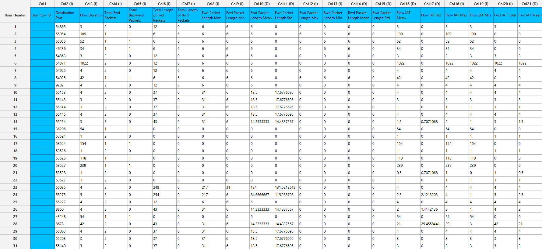
The data are inserted as shown below in the data input sheet on the left-hand side.

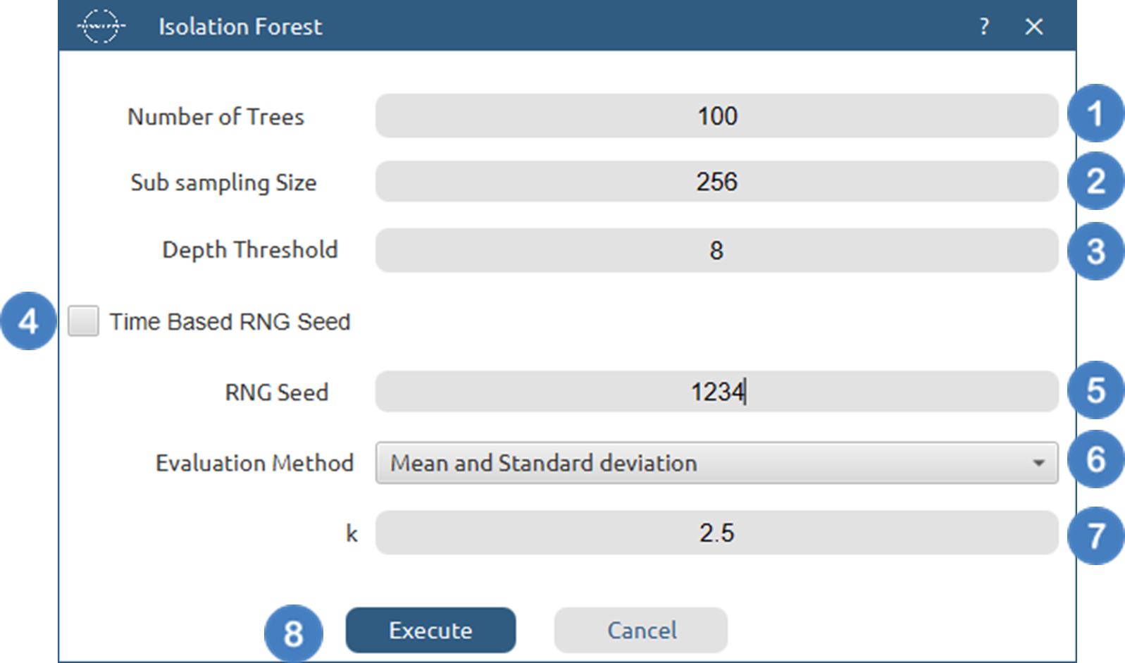
Configuration

1. Select Analytics → Anomaly Detection → Isolation Forest
2. Select the Number of Trees [1] to generate during the algorithm.
3. Select the Sub sampling Size [2]. Values should be integers smaller than the number of samples
4. Select the Depth Threshold [3] for each tree.
5. Select/tick to use a time based RNG Seed [4] or manually specify one[5].
6. Choose from the available option ther Evaluation Method [6] used to classify each data point as anomalous or normal.
7. Specify the parameter[7] for each of the Evaluation Method options.
8. Click on the Execute button [8] to apply the anomaly detection calculation.

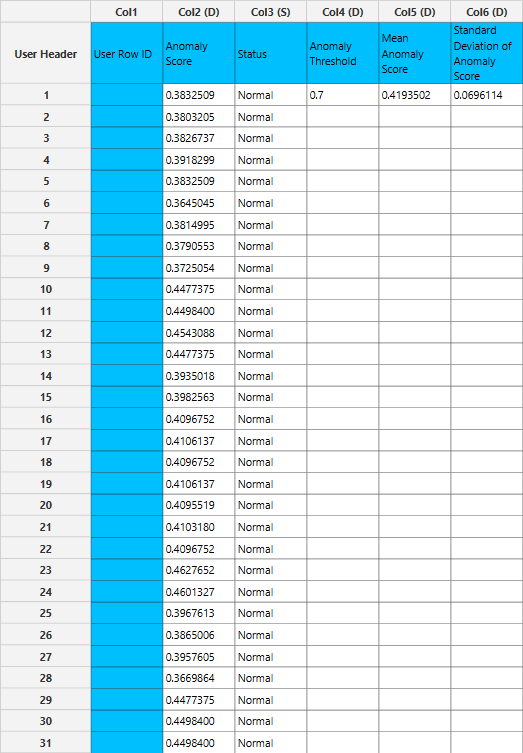
Output

The right-hand spreadsheet tab presents two columns in the output: one for predicting whether the result is normal or anomalous, and another for the scoring. The anomaly threshold along with the mean anomaly score and its standard deviation are also printed in columns 4-6.

References

1. Mehrotra, K.G., et al., Anomaly detection. 2017: Springer. doi.org/10.1007/978-3-319-67526-8.
2. Zhang, R., S. Zhang, S. Muthuraman, and J. Jiang. One class support vector machine for anomaly detection in the communication network performance data. in Proceedings of the 5th conference on Applied electromagnetics, wireless and optical communications. 2007. Citeseer. api.semanticscholar.org/CorpusID:111342328
3. F. T. Liu, K. M. Ting and Z. -H. Zhou, “Isolation Forest,” 2008 Eighth IEEE International Conference on Data Mining, Pisa, Italy, 2008, pp. 413-422 doi.org/110.1109/ICDM.2008.17.

---

Version History

Introduced in Isalos Analytics Platform v0.2.4

Instructions last updated on January 2025