Screening
Screening Designs are a subcategory under Design of Experiments (DoE), focused on identifying the most significant factors that influence a response variable before optimizing. These designs are used when there are many potential factors to consider, and the goal is to quickly determine which ones have a meaningful effect in order to preserve resources and minimize cost. By systematically varying multiple factors at different levels and analyzing their effects, screening designs help prioritize the factors that warrant further investigation in more detailed studies.
Plackett Burman
Plackett-Burman designs are an efficient and economical approach within the DoE framework, particularly tailored for screening large numbers of factors in a system, similar to the Fractional Factorial Design. These designs are used to explore the main effects of up to $𝑘 = 𝑁 − 1$ factors in $𝑁$ experimental runs, where $𝑁$ is a multiple of 4 (e.g., 8, 12, 16). Moreover, all factors should have exactly two levels which we call high(+) and low (-). This structure allows researchers to identify which factors have significant main effects while minimizing the number of experimental runs required. This method becomes invaluable in scenarios where a full factorial design would necessitate prohibitively large experiments, consuming excessive time and resources.
Plackett-Burman designs achieve their efficiency by maximizing the number of factors that can be evaluated in a minimal number of runs. Unlike fractional factorial designs, which are crafted to manage both main effects and interactions, Plackett-Burman designs are specifically focused on detecting main effects. They are classified as resolution III designs, meaning that while they are well-suited to identify main effects, they confound these main effects with two-factor interactions. This confounding is a calculated trade-off, as the design assumes that two-factor interactions are either negligible or of less interest in the preliminary stages of experimentation.
For instance, in a Plackett-Burman design with 12 runs, up to 11 factors can be investigated, and any two-factor interactions will be indistinguishable from the main effects. This arrangement is particularly useful when the goal is rapid screening to pinpoint which factors have the most influence on the response variable, rather than an exhaustive analysis of all interactions. When the number of runs is a power of two (e.g., 8 or 16), the Plackett-Burman design is identical to a resolution III fractional factorial design.
Plackett-Burman designs are exceptionally valuable in early-stage experiments where a large number of factors are present, but only a subset is likely to have a substantial impact on the outcome. In these situations, they provide a powerful means to filter out the less impactful factors, allowing researchers to focus subsequent experiments on the most promising candidates. By reducing the number of necessary experiments, Plackett-Burman designs offer a practical balance between resource efficiency and the acquisition of critical data, making them an indispensable tool in experimental research for system optimization and improvement.
Use the Plackett Burman designs by browsing in the top ribbon:
| DOE \(\rightarrow\) Screening \(\rightarrow\) Plackett Burman |
Input
Factor values must be specified in the input datasheet. The Plackett–Burman design is applied when at least three factors (columns) are provided. Factors may be either numerical or categorical. Categorical factors must contain exactly two distinct levels. Numerical factors may contain more than two values; in this case, the algorithm automatically determines the factor levels by taking the minimum and maximum values observed in the column.
Configuration
| Number of Center Points per Block | Select manually the Number of Center Points per Block to be included in the output list of experiments. There is no minimum requirement or any other limitation. When categorical factors are included in the analysis, the total number of center points is equal to the user-specified value multiplied by the number of possible combinations of categorical factor levels. |
| Number of Replicates | Select manually the Number of Replicates which represents the number of times to replicate the entire design. This value should be an integer, and the lowest acceptable value is 1. |
| Number of Blocks | Select from the list of available options the Number of Blocks. Plackett Burman designs can only be blocked on replicates, meaning each replicate defines a block, otherwise all points are put into a single block. |
| Random Standard order | You can tick/select the box if randomness is required in the output list of experiments. |
| Time-based RNG Seed | If the randomness is selected, then you have the option to also tick/select the box to set the random generated number seed based on time. |
| RNG Seed | Select manually the random generated number seed if required. |
| Include/exclude columns | Select manually the columns through the dialog window: Use the buttons to move columns between the Included Columns and Excluded Columns list. Single-arrow buttons will move all selected columns and double-arrow buttons will move all columns. |
| Number of Runs | Select from the available options the number of runs to produce. The available options include multiples of 4 starting from 8 until 48 that are larger than the number of selected factors. |
Output
A list of experiments (combinations) is generated in the output datasheet along with the Block number, the Replicate Number, the Standard order and the Point type of each experiment based on the Plackett-Burman design.
Example
Input
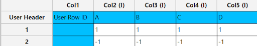
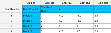
In the input datasheet minimum requirement is to specify three factors (columns) and insert exactly/minimum two levels (values) for each categorical/numerical factor (column), as shown below.
Configuration
- Select
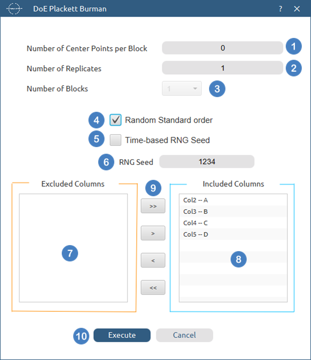
DOE\(\rightarrow\)Screening\(\rightarrow\)Plackett Burman. - Select the
Number of Center Points per Block[1] to be generated in the output list of experiments. - Select the
Number of Replicates[2]. The lowest value that can be set is 1. - Select the
Number of Blocks[3]. - Select/tick if required the
Random Standard order[4] to imply randomness in the output list of experiments. - If randomness is selected either select/tick to generate the number seed for randomness based on time [5] or by manually setting a value [6].
- Select the columns by clicking on the arrow buttons [9] and moving columns between the
Excluded Columns[7] andIncluded Columns[8] lists. - Select the
Number Of Runs[10] to produce. - Click on the
Executebutton [11] to perform Plackett-Burman design method.
Output
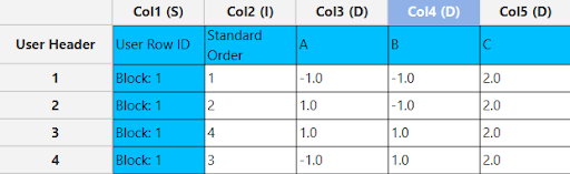
A list of experiments (combinations) is generated in the output datasheet along with the Block number based on the Plackett-Burman design method selected. Standard Order, Block number, Replicate Number and Point Type are presented in Cols 2,3,4 and 5 accordingly as shown below.
Definitive Screening
Definitive screening designs (DSDs) are a class of three-level screening designs intended for quantitative (continuous) factors when second-order effects (two-factor interactions and/or curvature) may be active. Their goal is to estimate main effects reliably while minimizing aliasing with second-order terms.
Traditional screening designs such as Plackett–Burman and many fractional factorial designs usually confound main effects with one or more two-way interactions. If a confounded effect is active, the experimenter cannot differentiate which of the confounded effects is responsible for the observed change in response. Therefore, it is crucial to have designs with a small number of runs that can be able to estimate main effects and second-order terms with minimal aliasing.
Here is where Definitive Screening Designs come into play. These designs require, in most cases, a number of runs only one more than twice the number of factors, thus making them highly efficient for screening purposes. Moreover, main effects are completely independent of two-factor interactions; two-factor interactions are not completely confounded with one another (although they may be correlated); and quadratic terms are estimable and orthogonal to main effects and not completely confounded with interaction effects.
In a Definitive Screening Design, each odd run has one factor at the mid level and all other factors at their extreme levels. Each even run is the multiplication by −1 (i.e., the reverse) of the previous odd run. This structure is finally enhanced with center points.
As described in [2], definitive screening designs can be constructed easily using conference matrices. For m even, an m*m matrix C is a conference matrix if it satisfies \(C^{'}C = (m-1)I\) with \(C_{ii} = 0\) and \(C_{ij} ∈ \{-1,1\}\) .
When m is even, we can use a conference matrix to construct a definitive screening design as \(D = {C \choose -C}\), while when m is odd, we delete the last row of an (m+1)*(m+1) conference matrix. If a conference matrix of the required size is not available, we use the next available conference matrix size and apply the same construction, deleting the extra column(s) as necessary to match the number of factors.
A table specifying the produced runs for each number of factors is shown below:
| Number of Factors | Produced Runs (Excluding center points) |
| 2- 6 | 12 |
| 7-8 | 16 |
| 9-10 | 20 |
| 11-12 | 24 |
| 13-14 | 28 |
| 15-16 | 32 |
| 17-18 | 36 |
| 19-20 | 40 |
| 21-24 | 48 |
| 25-26 | 52 |
| 27-30 | 60 |
| 31-32 | 64 |
| 33-38 | 76 |
| 39-42 | 84 |
| 43-44 | 88 |
| 45-48 | 96 |
Use the Definitive Screening designs by browsing in the top ribbon:
| DOE \(\rightarrow\) Screening \(\rightarrow\) Definitive Screening |
Input
Factor values must be specified in the input datasheet. The Plackett–Burman design is applied when at least two factors (columns) are provided. Factors may be either numerical or categorical. Categorical factors must contain exactly two distinct levels. Numerical factors may contain more than two values; in this case, the algorithm automatically determines the factor levels by taking the minimum and maximum values observed in the column.
Configuration
| Number of Center Points per Block | Specify the Number of Center Points per Block to be included in the generated list of experiments. There is no minimum requirement or upper limitation. For Definitive Screening Designs, center points are generated using the midpoint of all numerical factors, while categorical factors are set simultaneously to either their low level or their high level. Therefore, the number of center points is exactly equal to the user-specified value and is not multiplied by the number of categorical level combinations. |
| Number of Replicates | Select manually the Number of Replicates which represents the number of times to replicate the entire design. This value should be an integer, and the lowest acceptable value is 1. |
| Number of Blocks | Select from the list of available options the Number of Blocks. Plackett Burman designs can only be blocked on replicates, meaning each replicate defines a block, otherwise all points are put into a single block. |
| Random Standard order | You can tick/select the box if randomness is required in the output list of experiments. |
| Time-based RNG Seed | If the randomness is selected, then you have the option to also tick/select the box to set the random generated number seed based on time. |
| RNG Seed | Select manually the random generated number seed if required. |
| Include/exclude columns | Select manually the columns through the dialog window: Use the buttons to move columns between the Included Columns and Excluded Columns list. Single-arrow buttons will move all selected columns and double-arrow buttons will move all columns. |
Output
A list of experiments (combinations) is generated in the output datasheet along with the Block number, the Replicate Number, the Standard order and the Point type of each experiment based on the Definitive Screening design.
Example
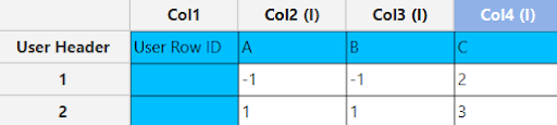
Input
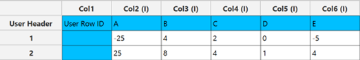
In the input datasheet minimum requirement is to specify two factors (columns) and insert exactly/minimum two levels (values) for each categorical/numerical factor (column), as shown below.
Configuration
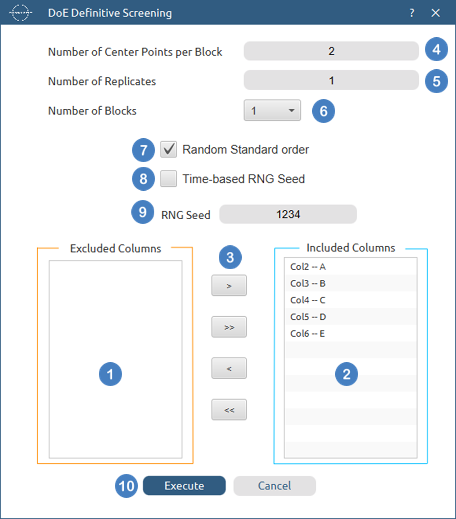
- Select
DOE\(\rightarrow\)Screening\(\rightarrow\)Definitive-Screening. - Select the
Number of Center Points per Block[1] to be generated in the output list of experiments. - Select the
Number of Replicates[2]. The lowest value that can be set is 1. - Select the
Number of Blocks[3]. - Select/tick if required the
Random Standard order[4] to imply randomness in the output list of experiments. - If randomness is selected either select/tick to generate the number seed for randomness based on time [5] or by manually setting a value [6].
- Select the columns by clicking on the arrow buttons [9] and moving columns between the
Excluded Columns[7] andIncluded Columns[8] lists. - Click on the
Executebutton [10] to perform Plackett-Burman design method.
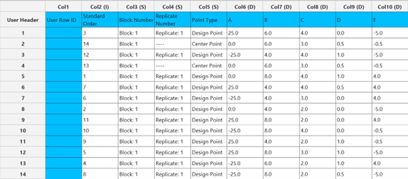
Output
A list of experiments (combinations) is generated in the output datasheet along with the Block number based on the Definitive Screening design method selected. Standard Order, Block number, Replicate Number and Point Type are presented in Cols 2,3,4 and 5 accordingly as shown below.
Fractional Factorial
Fractional factorial designs represent a refined approach within the framework of DoE that addresses the challenge of studying systems with multiple factors without resorting to the exhaustive method used in full factorial designs. By selectively sampling a fraction of the full factorial design, these designs allow researchers to explore the effects of various factors using a substantially reduced number of experimental runs. This method is particularly valuable when dealing with a large number of factors, where a full factorial design would require an impractically large set of experiments, escalating costs and resource usage.
The efficiency of fractional factorial designs comes from their strategic choice of factor level combinations, capturing essential information about the system while significantly cutting down on the number of required experiments. This efficiency, however, introduces the primary challenge of confounding. Confounding occurs when the effects of some factor combinations become indistinguishable from others. For instance, in a four-factor experimental setup, a typical confounding pattern such as “A - B - C - BC” implies that the effect of the fourth factor is entangled with the combined effects of the second and third factors. This overlap means that while the design is more efficient, it sacrifices some ability to precisely attribute effects to individual factors or their specific combinations.
Despite this trade-off, with meticulous design and a clear understanding of the system under study, fractional factorial designs can yield significant insights. They are particularly adept at identifying the main effects and certain interactions among the factors, which are often sufficient for preliminary analysis or when certain factors or interactions are suspected to be of lesser importance.
Moreover, fractional factorial designs prove exceptionally useful in scenarios where some factors are presumed to have minimal or no effect, or where certain interactions are deemed negligible. In these cases, the designs can provide nearly as comprehensive information as full factorial designs but at a fraction of the operational cost and effort. This makes fractional factorial designs a highly strategic tool in experimental research, balancing resource management with the acquisition of critical data points necessary for effective decision-making in system optimization and improvement.
Isalos uses a term called “Fraction Relationship” to determine the confounding pattern the user wishes to use. The “Fraction Relationship” is a sequence of strings, separated by spaces, where the $k^{th}$ string specifies how the $k^{th}$ factor is confounded. If a factor is not confounded with any other, it is represented by its corresponding single letter. For example, when conducting an experiment with 5 factors which we denote A, B, C, D and E, a valid “Fraction Relationship” would be “A B C AB AC” which determines that D = AB and E=AC.
Resolution measures the extent to which effects—such as main effects and interactions between factors—can be uniquely estimated without confounding. It is determined by the shortest word in the defining relation of the design, which represents the smallest group of factors whose effects are confounded. The minimum acceptable resolution for a design is Resolution III, as resolutions below this result in main effects being confounded with one another, which is undesirable for meaningful analysis.
To assist users in determining the required “Fraction Relationship,” the software provides a comprehensive list of available designs that deliver maximum resolution for each case. These designs serve as a reliable reference, derived from authoritative sources 3, 4, 5 and can be used by selecting one of the options from the Available Designs. However, users can also specify a different fraction relationship by selecting the Custom Option.
| Number of Factors | Fraction | Number of Runs | Design Generators | Fraction Relationship | Resolution |
|---|---|---|---|---|---|
| 3 | “1/2” | 4 | c=ab | a b ab | III |
| 4 | “1/2” | 8 | d=abc | a b c abc | IV |
| 5 | “1/2” | 16 | e=abcd | a b c d abcd | V |
| “1/4” | 8 | d=ab, e=ac | a b c ab ac | III | |
| 6 | “1/2” | 32 | f=abcde | a b c d e abcde | VI |
| “1/4” | 16 | e=abc, f=bcd | a b c d abc bcd | IV | |
| “1/8” | 8 | d=ab, e=ac, f=bc | a b c ab ac bc | III | |
| 7 | “1/2” | 64 | g=abcdef | a b c d e f abcdef | VII |
| “1/4” | 32 | f=abcd, g=abde | a b c d e abcd abde | IV | |
| “1/8” | 16 | e=abc, f=bcd, g=acd | a b c d abc bcd acd | IV | |
| “1/16” | 8 | d=ab, e=ac, f=bc, g=abc | a b c ab ac bc abc | III | |
| 8 | “1/2” | 128 | h=abcdefg | a b c d e f g abcdefg | VIII |
| “1/4” | 64 | g=abcd, h=abef | a b c d e f abcd abef | V | |
| “1/8” | 32 | f=abc, g=abd, h=bcde | a b c d e abc abd bcde | IV | |
| “1/16” | 16 | e=bcd, f=acd, g=abc, h=abd | a b c d bcd acd abc abd | IV | |
| 9 | “1/2” | 256 | i=abcdefgh | a b c d e f g h abcdefgh | IX |
| “1/4” | 128 | h=acdfg, i=bcefg | a b c d e f g acdfg bcefg | VI | |
| “1/8” | 64 | g=abcd, h=acef, i=cdef | a b c d e f abcd acef cdef | IV | |
| “1/16” | 32 | f=bcde, g=acde, h=abde, i=abce | a b c d e bcde acde abde abce | IV | |
| “1/32” | 16 | e=abc, f=bcd, g=acd, h=abd, i=abcd | a b c d abc bcd acd abd abcd | III | |
| 10 | “1/2” | 512 | j=abcdefghi | a b c d e f g h i abcdefghi | X |
| “1/8” | 128 | h=abcg, i=bcde, j=acdf | a b c d e f g abcg bcde acdf | V | |
| “1/16” | 64 | g=bcdf, h=acdf, i=abde, j=abce | a b c d e f bcdf acdf abde abce | IV | |
| “1/32” | 32 | f=abcd, g=abce, h=abde, i=acde, j=bcde | a b c d e abcd abce abde acde bcde | IV | |
| “1/64” | 16 | e=abc, f=bcd, g=acd, h=abd, i=abcd, j=ab | a b c d abc bcd acd abd abcd ab | III | |
| 11 | “1/2” | 1024 | k=abcdefghij | a b c d e f g h i j abcdefghij | XI |
| “1/16” | 128 | h=abcg, i=bcde, j=acdf, k=abcdefg | a b c d e f g abcg bcde acdf abcdefg | V | |
| “1/32” | 64 | g=cde, h=abcd, i=abf, j=bdef, k=adef | a b c d e f cde abcd abf bdef adef | IV | |
| “1/64” | 32 | f=abc, g=bcd, h=cde, i=acd, j=ade, k=bde | a b c d e abc bcd cde acd ade bde | IV | |
| “1/128” | 16 | e=abc, f=bcd, g=acd, h=abd, i=abcd, j=ab, k=ac | a b c d abc bcd acd abd abcd ab ac | III | |
| 12 | “1/2” | 2048 | l=abccdefghijk | a b c d e f g h i j k abccdefghijk | XII |
| “1/32” | 128 | h=acdg, i=abcd, j=bcfg, k=abcdefg, l=cdef | a b c d e f g acdg abcd bcfg abcdefg cdef | IV | |
| “1/64” | 64 | g=def, h=abc, i=bcde, j=bcdf, k=abef, l=acef | a b c d e f def abc bcde bcdf abef acef | IV | |
| “1/128” | 32 | f=ace, g=acd, h=abd, i=abe, j=cde, k=abcde, l=ade | a b c d e ace acd abd abe cde abcde ade | IV | |
| “1/256” | 16 | e=abc, f=abd, g=acd, h=bcd, i=abcd, j=ab, k=ac, l=ad | a b c d abc abd acd bcd abcd ab ac ad | III | |
| 13 | “1/2” | 4096 | m=abcdefghijkl | a b c d e f g h i j k l abcdefghijkl | XIII |
| “1/64” | 128 | h=defg, i=bceg, j=bcdfg, k=abdef, l=acef, m=abc | a b c d e f g defg bceg bcdfg abdef acef abc | IV | |
| “1/128” | 64 | g=abc, h=def, i=bcdf, j=bcde, k=abef, l=acef, m=bcef | a b c d e f abc def bcdf bcde abef acef bcef | IV | |
| “1/256” | 32 | f=ace, g=bce, h=abc, i=cde, j=abcde, k=abe, l=acd, m=ade | a b c d e ace bce abc cde abcde abe acd ade | IV | |
| “1/512” | 16 | e=abc, f=abd, g=acd, h=bcd, i=abcd, j=ab, k=ac, l=ad, m=bc | a b c d abc abd acd bcd abcd ab ac ad bc | III | |
| 14 | “1/2” | 8192 | n=abcdefghijklm | a b c d e f g h i j k l m abcdefghijklm | XIV |
| “1/128” | 128 | h=efg, i=bcfg, j=bceg, k=abef, l=acef, m=bcdef, n=abc | a b c d e f g efg bcdg bceg abef acef bcdef abc | IV | |
| “1/256” | 64 | g=bef, h=bcf, i=def, j=cef, k=bce, l=cdf, m=acde, n=bcdef | a b c d e f bef bcf def cef bce cdf acde bcdef | IV | |
| “1/512” | 32 | f=abc, g=abd, h=abe, i=acd, j=ace, k=ade, l=bcd, m=bce, n=bde | a b c d e abc abd abe acd ace ade bcd bce bde | IV | |
| “1/1024” | 16 | e=abc, f=abd, g=acd, h=bcd, i=abcd, j=ab, k=ac, l=ad, m=bc, n=bd | a b c d abc abd acd bcd abcd ab ac ad bc bd | III | |
| 15 | “1/2” | 16384 | o=abcdefghijklmn | a b c d e f g h i j k l m n abcdefghijklmn | XV |
| “1/256” | 128 | h=abfg, i=acdef, j=bef, k=abcdeg, l=cdfg, m=acdeg, n=efg, o=abdefg | a b c d e f g abfg acdef bef abcdeg cdfg acdeg efg abdefg | IV | |
| “1/512” | 64 | g=abc, h=abd, i=abe, j=bcde, k=acf, l=adf, m=aef, n=cdef, o=abcdef | a b c d e f abc abd abe bcde acf adf aef cdef abcdef | IV | |
| “1/1024” | 32 | f=abc, g=abd, h=abe, i=acd, j=ace, k=ade, l=bcd, m=bce, n=bde, o=cde | a b c d e abc abd abe acd ace ade bcd bce bde cde | IV | |
| “1/2048” | 16 | e=abc, f=abd, g=acd, h=bcd, i=abcd, j=ab, k=ac, l=ad, m=bc, n=bd, o=cd | a b c d abc abd acd bcd abcd ab ac ad bc bd cd | III |
Moreover, Isalos offers the option to orthogonally block fractional factorial designs based on block generators found in literature.3
Use the Fractional Factorial function by browsing in the top ribbon:
| DOE \(\rightarrow\) Screening \(\rightarrow\) Fractional Factorial |
Input
Factor values must be specified in the input datasheet. The Fractional-Factorial design is applied when at least three factors (columns) are provided. Factors may be either numerical or categorical. Categorical factors must contain exactly two distinct levels. Numerical factors may contain more than two values; in this case, the algorithm automatically determines the factor levels by taking the minimum and maximum values observed in the column.
Configuration
| Available Designs | Select one of the available design options for the number of factors you have selected. Choices include the fraction of the produced design, while the fraction relationship being used maximizes the resolution of the design. There is also the option to specify a custom design. |
| Fraction Relationship | If the Custom option is selected from the Available Designs, insert manually the Fraction Relationship to define the desired Fractional Factorial design. The kth independent factor(column) corresponds to the kth letter of the alphabet (The letter I is not a special character and should be used for the 9th if that exists). Only alphabetical characters, spaces, ‘+’ and ‘-‘ are allowed. |
| Number of Center Points per Block | Select manually the Number of Center Points per Block to be included in the output list of experiments. There is no minimum requirement or any other limitation. When categorical factors are included in the analysis, the total number of center points is equal to the user-specified value multiplied by the number of possible combinations of categorical factor levels. |
| Number of Replicates | Select manually the Number of Replicates which represents the number of times to replicate the entire design. This value should be an integer, and the lowest acceptable value is 1. |
| Number of Blocks | Select from the list of available options the Number of Blocks. Available options depend on the selected number of factors, the selected design and the number of replicates. |
| Random Standard order | You can tick/select the box if randomness is required in the output list of experiments. |
| Time-based RNG Seed | If in the randomness is selected, then you have the option to also tick/select the box to set the random generated number seed based on time |
| RNG Seed | Select manually the random generated number seed if required. |
| Include/exclude columns | Select manually the columns through the dialog window: Use the buttons to move columns between the Included Columns and Excluded Columns list. Single-arrow buttons will move all selected columns and double-arrow buttons will move all columns. |
Output
A list of experiments (combinations) is generated in the output datasheet along with the Block number, the Replicate Number, the Standard order and the Point type of each experiment based on the Fractional Factorial design method selected.
Example
Input
In the input datasheet minimum requirement is to specify three factors (columns) and insert exactly/minimum two levels (values) for each categorical/numerical factor (column), as shown below.
Configuration
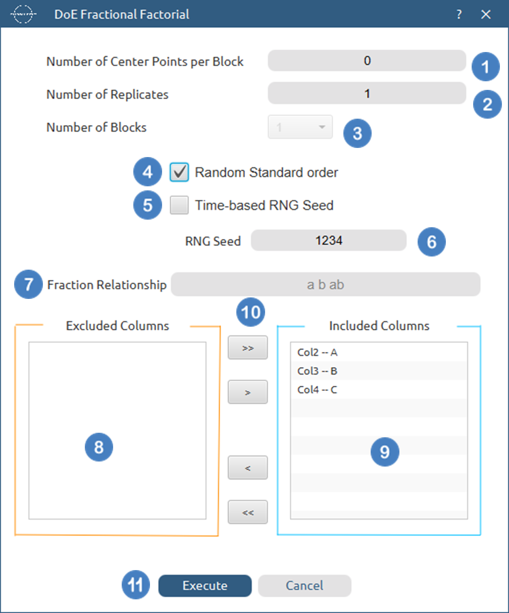
- Select
DOE\(\rightarrow\)Screening\(\rightarrow\)Fractional Factorial. - Select the columns by clicking on the arrow buttons [3] and moving columns between the
Excluded Columns[1] andIncluded Columns[2] lists. - Select one
of the Available Designs[4]. - If the Custom option is selected, insert the
Fraction Relationship[5]. - Select the
Number of Center Points per Block[6] to be generated in the output list of experiments. - Select the
Number of Replicates[7]. The lowest value that can be set is 1. - Select the
Number of Blocks[8]. - Select/tick if required the
Random Standard order[9] to imply randomness in the output list of experiments. - If randomness is selected either select/tick to generate the number seed for randomness based on time [10] or by manually setting a value [11].
- Click on the
Executebutton [12] to perform Fractional Factorial design method.
Output
A list of experiments (combinations) is generated in the output datasheet along with the Block number based on the Fractional Factorial design method selected. Standard Order, Block number, Replicate Number and Point Type are presented in Cols 2,3,4 and 5 accordingly as shown below.
References
-
Box, G.E. and Behnken, D.W., Some new three level designs for the study of quantitative variables. Technometrics, 1960. 2(4): p. 455-475. doi.org/10.1080/00401706.1960.10489912.
-
Box, G.E. and Wilson, K.B., On the experimental attainment of optimum conditions, in Breakthroughs in statistics: methodology and distribution. 1992, Springer. p. 270-310. doi.org/10.1007/978-1-4612-4380-9_23.
-
Montgomery, Douglas C. Design and analysis of experiments. John wiley & sons, 2017.
-
Speed, Terry. Statistics for Experimenters: Design, Innovation, and Discovery. 2006.
-
Wu, CF Jeff, and Michael S. Hamada. Experiments: planning, analysis, and optimization. John Wiley & Sons, 2011.
-
Jones, Bradley, and Christopher J. Nachtsheim. “A class of three-level designs for definitive screening in the presence of second-order effects.” Journal of Quality Technology 43, no. 1 (2011): 1-15.
-
Xiao, Lili, Dennis KJ Lin, and Fengshan Bai. “Constructing definitive screening designs using conference matrices.” Journal of Quality Technology 44, no. 1 (2012): 2-8.
Version History
Introduced in Isalos Analytics Platform v0.2.4
Instructions last updated on November 2025