Regression
Regression is a typical supervised learning task in predictive modelling that aims to investigate the relationship between a set of independent features and a dependent target variable. Regression analysis algorithms are employed when the target variable is a continuous numeric value.1
k Nearest Neighbors (kNN)
k Nearest Neighbors (kNN) is a simple non-parametric algorithm that operates by identifying the data points from the training set that are most proximate to a new unseen input. This instance-based learning method determines the closeness of data points by calculating the Euclidean distance between instances considering all attribute values. The k parameter denotes the number of nearest neighbors to consider.2 The target value for a new instance is predicted by averaging the distance-weighted target values of the k nearest data points. As calculations of Euclidean distances are performed, scaling of data is performed within the function.
Use the k Nearest Neighbors (kNN) function by browsing in the top ribbon:
| Analytics \(\rightarrow\) Regression \(\rightarrow\) k Nearest Neighbors (kNN) |
Input
Data matrix with training set data.
Configuration
| Target Column | Select from the drop-down menu the column containing the target variable that is going to be predicted. Columns with categorical features cannot be selected as targets. |
| Number of Neighbors | An integer representing the number of closest neighbours-data points (k) used to make predictions for a new data point. |
Output
A data matrix including the actual target value and the value predicted by the algorithm (“kNN Prediction”). For each data point, the closest neighbors from the training set are listed in the “Closest NN” columns, along with their corresponding distances in the “Distance from NN” columns.
Example
Input
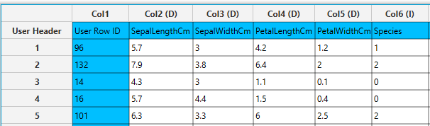
In the left-hand spreadsheet of the tab import the data matrix including the target variable for prediction.
Configuration
- Select
Analytics\(\rightarrow\)Regression\(\rightarrow\)k Nearest Neighbors (kNN). - Select the column that is going to be predicted from the drop-down menu [1]. The columns containing categorical features are automatically excluded from the list.
- Type the
Number of Neighbors[2] to consider. - Click on the
Executebutton [3] to apply the algorithm on the input table.

Output
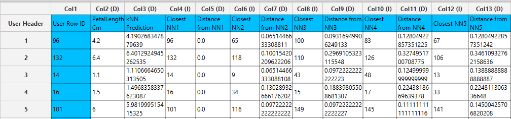
In the right-hand spreadsheet of the tab the output data matrix with the actual and the predicted value of the target is presented. Also, the k most proximate identified instances from the training set are given for each data point (5 in this case), along with the corresponding Euclidean distances from each neighbor. Note that the “Closest NN1” represents the nearest neighbor, which is the data point itself when applied on the training set. Consequently, the “Distance from NN1” is 0 for all given training instances.
Application on external set
You can apply the trained k Nearest Neighbors (kNN) model to any external (test) data using the Existing Model Utilization function:
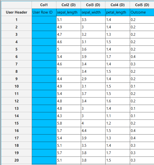
- Import the external data in the left-hand spreadsheet of the tab. Include the same columns used to build the kNN model.
- Select
Analytics\(\rightarrow\)Existing Model Utilization. Select the trained kNN model [1] and click on theExecutebutton [2].

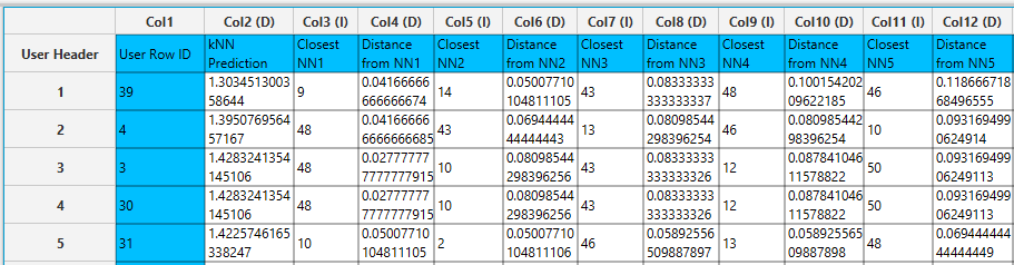
- Inspect the results in the right-hand spreadsheet of the tab. Note that in this case the closest neighbor listed in the “Closest NN1” belongs to the training set, and the “Distance from NN1” is not zero.
Fully Connected Neural Network
A type of feedforward artificial neural network consisting of multiple layers of neurons. It consists of an input layer, one or more hidden layers and an outer layer, which are fully connected with each other. A variety of non-linear activation functions are typically used in the hidden layer, allowing the network to learn complex patterns in data. MLP uses a backpropagation algorithm to train the model and classify instances.1,2
Use the Fully Connected Neural Network function by browsing in the top ribbon:
| Analytics \(\rightarrow\) Regression \(\rightarrow\) Fully Connected Neural Network |
Input
Data matrix with training set data. String columns are not taken into account in the algorithm implementation, therefore categorical features must be removed or encoded into numerical values.
Configuration
| Batch Size | Select from the drop-down menu the number of training instances that will be propagated through the network. Four options are available for selection: 16, 32, 64, and 128. |
| Number of Epochs | Specify the number (integer) of complete passes through the data during training. |
| Learning Rate | Specify the learning rate (between 0 and 1), which controls the size of the steps taken during optimization. |
| Momentum | Specify the momentum rate (between 0 and 1) for the backpropagation algorithm. |
| +/- | Click on the + and - buttons to add or remove hidden layers, respectively. |
| Hidden Layers | For each added hidden layer, specify the number of neurons and select the non-linear activation function used to map the weighted inputs to the output of each neuron. Options for the activation functions include: - RELU, - RELU6, - LEAKYRELU, - SELU, - SWISH, - RRELU, - SIGMOID, - SOFTMAX, - SOFTPLUS, - SOFTSIGN, - TANH, - THRESHOLDEDRELU, - GELU, - ELU, - MISH, - CUBE, - HARDSIGMOID, - HARDTANH, - IDENTITY, - RATIONALTANH, and - RECTIFIEDTANH. |
| Target Column | Select from the drop-down menu the column containing the feature that is going to be predicted. |
| RNG Seed | Select an integer as seed to get reproducible results. The option to select a time-based random number-generated seed is available. |
Output
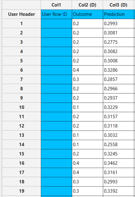
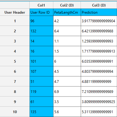
A data matrix including the actual target value and the value predicted by the algorithm (“Prediction”) is presented.
Example
Input
In the left-hand spreadsheet of the tab import the data matrix including the target variable with at least two distinct categories for prediction. In case that categorical-string columns are included in the set, these should be encoded into representative numerical values.
Configuration
- Select
Analytics\(\rightarrow\)Regression\(\rightarrow\)Fully Connected Neural Network - Select the hyperparameters that determine the training procedure: the
Batch Size[1], theNumber of Epochs[2], theLearning Rate[3] and theMomentum[4]. - Select the hyperparameters that determine the
Hidden Layers[5] of the neural network: the number of neurons [6] and the activation function [7] of each layer. - Add [8] or remove [9] hidden layers to define the architecture of the neural network.
- Select the column that is going to be predicted from the drop-down menu [10].
- Select a Seed for reproducible results or a random number generated
Time-based (RNG) Seed[11]. - Click on the
Executebutton [12] to apply the training algorithm on the input columns.

Output
In the right-hand spreadsheet of the tab the output data matrix with the actual and the predicted values of the target is presented.
Radial Basis Function Network
Radial basis function (RBF) network is an artificial neural network that employs RBF kernels as activation functions. The network consists of three layers: the input layer modeling a vector that passes data, the hidden layer that performs computations and the output layer designated for regression problems. The output layer of the neural network is a linear combination of the activation (output) from the hidden units.1, 3
A Radial Basis Function is a real-valued function $φ(r)$ that is dependent only on the distance between a fixed input point ($r$) to the center ($c$) of each neuron as reference point Eq. 1.3
The radial basis function kernels available in Isalos include:
Gaussian:
Multiquadric:
Inverse Quadratic:
Inverse Multiquadric:
Polyharmonic spline:
where $k$ is the order of the spline.
Thin Plate Spline:
Bump Function:
where $\varepsilon$ is the shape parameter used to scale the input of the radial kernel.
Use the Radial Basis Function Network regression function by browsing in the top ribbon:
| Analytics \(\rightarrow\) Regression \(\rightarrow\) Radial Basis Function Network |
Input
Data matrix with training set data. String columns are not taken into account in the algorithm implementation, therefore categorical features must be removed or encoded into numerical values. RBF does not allow the use of integer or string input.
Configuration
| Hidden Neurons | Specify the number of neurons in the hidden layer of the network. |
| RBF Kernel | Select from the drop-down menu the radial basis function kernel. Options include: - GAUSSIAN Eq. 2, - MULTIQUADRIC Eq. 3, - INVERSE QUADRATIC Eq. 4, - INVERSE MULTIQUADRIC Eq. 5, - POLYHARMONIC SPLINE Eq. 6, - THIN PLATE SPLINE Eq. 7, and - BUMP FUNCTION Eq. 8. A new configuration field appears accordingly after RBF Kernel selection, for the selection of Epsilon ($\varepsilon$) shape parameter or K ($k$) where applicable. |
| Point Selection | Select manually the way that determines how the centers of the neural network are chosen. Options include: - Random Points from Training set: chosen randomly from the training data. - Use KMeans: RBF centers are the cluster centers of the partitioned training data. |
| RNG Seed | Select an integer as seed to get reproducible results. The option to select a time-based random number-generated seed is available. |
| Target Column | Select from the drop-down menu the column containing the target variable that is going to be predicted. Columns with categorical features cannot be selected as targets. |
Output
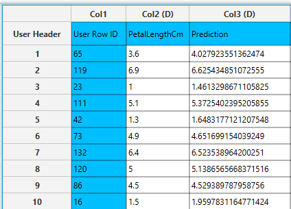
A data matrix including the actual target value and the value predicted by the algorithm (“Prediction”) is presented.
Example
Input
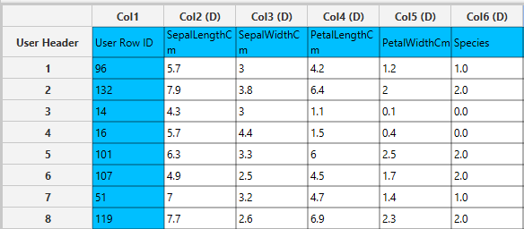
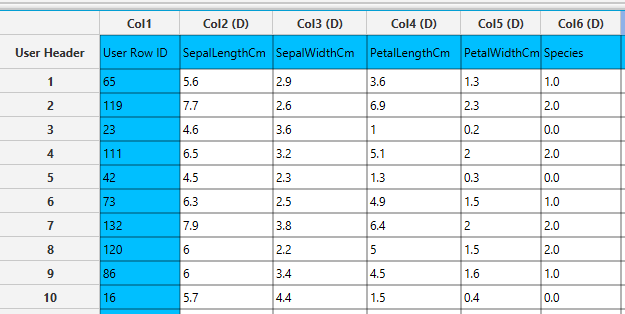
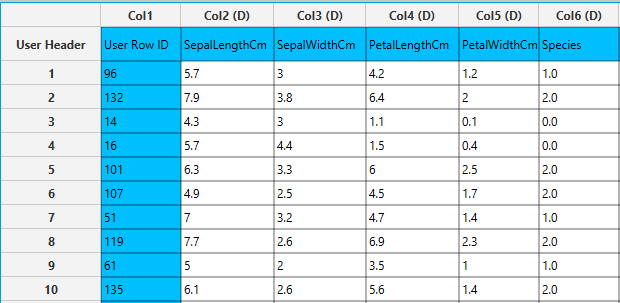
In the left-hand spreadsheet of the tab import the data matrix including the target variable for prediction. Note that the “Species” categorical column is presented as double (D).
Configuration
- Select
Analytics\(\rightarrow\)Regression\(\rightarrow\)Radial Basis Function Network - Type the number (integer) of
Hidden Neurons[1]. - Select the
RBF Kernel[2] used as activation function of the hidden layer and subsequently select theEpsilon[3] orKparameter where applicable. - Select the
Point Selection[4] method to determine the center of the network. - Type an
RNG Seedfor reproducible results or a random number generatedTime-based (RNG) Seed[5]. - Select the
Target Columnthat is going to be predicted from the drop-down menu [6]. Columns with categorical features cannot be selected as targets. - Click on the
Executebutton [7] to proceed with training.

Output
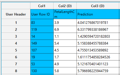
In the right-hand spreadsheet of the tab the output data matrix with the actual and the predicted value of the target variable is presented.
Linear SGD
Stochastic Gradient Descent (SGD) is a method used to minimize an objective (loss) function, which measures the error between the actual values and the predicted outcomes of data points. SGD is employed to incrementally fit various linear regressors by iteratively updating the parameters of a linear model. At each step, it estimates the gradient of the loss function and adjusts the parameters using a constant or decreasing learning rate. Unlike traditional gradient descent, which processes the entire training set in each iteration, SGD operates on a small batch of the training data, enabling faster convergence.1,5
Use the Linear SGD regression function by browsing in the top ribbon:
| Analytics \(\rightarrow\) Regression \(\rightarrow\) Linear SGD |
Input
Data matrix with training set data. String columns are not taken into account in the algorithm implementation, therefore categorical features must be removed or encoded into numerical values. Linear SGD does not allow the use of integer or string input.
Configuration
| Target Column | Select from the drop-down menu the column containing the target variable that is going to be predicted. Columns with categorical features cannot be selected as targets. |
| Loss function | Select manually from the drop-down menu the objective function to be minimized. Three options are available for selection, namely: - Squared Loss: average of the squared errors, - Absolute Loss: average of the absolute differences, and - Huber Loss: combination of Squared Loss and Absolute Loss. |
| Optimizer | Select manually the gradient optimizer from the drop-down menu. Three options are available for selection, namely: - Linear Decay SGD: decreasing learning rate over time - Simple SGD: constant learning rate through training - Squared Root Decay SGD: learning rate is decreasing inversely to the number of iterations. |
| Learning rate | Specify the initial step size (between 0 and 1) used in the iterative optimization procedure (default value: 0.1). |
| Number of epochs | Specify the number (integer) of complete passes through the data during training (default value: 10). |
| RNG Seed | Select an integer as seed to get reproducible results. The option to select a time-based random number-generated seed is available. |
Output
A data matrix including the actual target value and the value predicted by the algorithm (“Prediction”) is presented.
Example
Input
In the left-hand spreadsheet of the tab import the data matrix including the target variable for prediction. Note that the “Species” categorical column is presented as double (D).
Configuration
- Select
Analytics\(\rightarrow\)Regression\(\rightarrow\)Linear SGD. - Select the column containing the target variable that is going to be predicted from the drop-down menu [1]. Columns with categorical features cannot be selected as targets.
- Select the
Loss function[2] and the gradientOptimizer[3] from the drop-down menus. - Type the hyperparameters that determine the structure of the model: the
Learning rate[4] and theNumber of epochs[5]. Default values, data types (double or integer) and acceptable ranges are indicated as guidance on the input parameter values. - Type an
RNG Seedfor reproducible results or a random number generatedTime-based (RNG) Seed[6]. - Click on the
Executebutton [7] to apply the training algorithm on the input data.

Output
In the right-hand spreadsheet of the tab the output data matrix with the actual and the predicted value of the target is presented.
XGBoost
The Extreme Gradient Boosting (XGBoost) open-source library6 is used to implement the gradient boosting framework. The library uses a class of ensemble machine learning algorithms constructed from decision tree models. Ensemble learning operates by combining different individual base learners to obtain a final prediction.7 In an iterative process, trees are added to the ensemble so that the prediction error (loss) of previous models is reduced. In regression problems, the mean squared error is used as loss function.8
Use the XGBoost regression function by browsing in the top ribbon:
| Analytics \(\rightarrow\) Regression \(\rightarrow\) XGBoost |
Input
Data matrix with training set data. String columns are not taken into account in the algorithm implementation, therefore categorical features must be removed or encoded into numerical values (integer or double).
Configuration
| Target Column | Select from the drop-down menu the column containing the target variable that is going to be predicted. Columns with categorical features cannot be selected as targets. |
| booster | Select from the drop-down menu which booster to use. Three options are available for selection, namely: - gbtree: default tree-based models, - dart: tree-based models, and - gblinear: linear functions. |
| objective | Select from the drop-down menu the learning objective of the method. Options include: - reg:squarederror: regression with squared loss, - reg:gamma: gamma regression with log-link, whose output is a mean of gamma distribution, and - reg:tweedie: tweedie regression with log-link. |
| number of estimators | Type the number of models (integer) to train in the learning ensemble. |
| eta | Specify the learning rate (between 0 and 1) which determines the step size shrinkage to prevent overfitting (default value: 0.3). |
| gamma | Specify the minimum loss reduction required to make a further partition on a leaf node of the tree (default value: 0). |
| max depth | Specify the maximum depth of a tree as a positive integer (default value: 6). |
| min child weight | Specify the minimum sum of instance weight (hessian) needed in a child (default value: 1). |
| column sample by tree | Specify the subsample ratio of features when constructing each tree. Subsampling will occur once for every tree constructed. |
| sub sample | Specify the subsampling ratio (between 0 and 1) of the training instances. Subsampling will occur once in every boosting iteration (default value: 1). |
| tree method | Select the tree construction algorithm used in XGBoost. Options include: - auto: use this heuristically to choose the fastest method typically based on the dataset size, - exact: exact greedy algorithm, - approx: approximates the greedy algorithm using quantile sketch and gradient histogram, and - hist: fast histogram optimized approximate greedy algorithm. |
| lambda | Specify the L2 regularization term on leaf weights (default value: 1). |
| alpha | Specify the L1 regularization term on leaf weights (default value: 0). |
| RNG Seed | Select an integer as seed to get reproducible results. The option to select a time-based random number-generated seed is available by clicking on the Time-based RNG Seed checkbox. |
Output
A data matrix including the actual target value and the value predicted by the algorithm (“Prediction”) is presented.
Example
Input
In the left-hand spreadsheet of the tab import the data matrix including the target variable for prediction. Note that the “Species” categorical column is presented as double (D).
Configuration
- Select
Analytics\(\rightarrow\)Regression\(\rightarrow\)XGBoost. - Select the column that is going to be predicted from the drop-down menu [1].
- Select the tree
booster[2] method, theobjectivefunction [3] for loss and type thenumber of estimators[4] involved in the ensemble. - Select the hyperparameters involved in the regularization of the model:
eta[5],gamma[6],lambda[12] andalpha[13]. Select the hyperparameters involved in tree construction:max depth[7] andmin child weight[8]. Select the column sampling rate by tree [9] and the overall subsampling rates [10]. Default values, data types (double or integer) and acceptable ranges are indicated as guidance on the input parameter values. - Select the tree construction algorithm [11] used in the XGBoost.
- Type an
RNG Seedfor reproducible results or a random number generatedTime-based RNG Seed[14]. - Click on the
Executebutton [15] to apply the training algorithm on the input data.

Output
In the right-hand spreadsheet of the tab the output data matrix with the actual and the predicted value of the target variable is presented.
Random Forest
Random forest regressor is an ensemble learning method that operates by building multiple randomized decision trees during training and obtaining the prediction of the individual trees. The decision trees are constructed in parallel, with no interaction between them, using random subsets of training data and input attributes to ensure diversity. Predictions independently made by all the trees in the forest are aggregated and averaged to produce a final prediction.7,9
Use the Random Forest function by browsing in the top ribbon:
| Analytics \(\rightarrow\) Regression \(\rightarrow\) Random Forest |
Input
Data matrix with training set data. String columns are not taken into account in the algorithm implementation, therefore categorical features must be excluded or encoded into numerical values (integer or double).
Configuration
| Features fraction | Specify the feature subsampling rate represented as a fraction of features (between 0 and 1) available in each tree split (default value: 0.9). |
| Min impurity decrease | Specify the impurity decrease threshold (between 0 and 1) necessary to determine the quality of splits in the decision trees. A split is only considered if it results in a decrease of impurity greater than or equal to this value (default value: 0.1). |
| Seed | Select an integer as seed to get reproducible results. The option to select a time-based random number-generated seed is available. |
| Number of ensembles | Specify the number of individual trees to be generated by the algorithm (default value: 10). |
| Target column | Select manually from the drop-down menu the column name containing the target variable that is going to be predicted. |
Output
A data matrix including the actual target value and the value predicted by the algorithm (“Prediction”) is presented.
Example
Input
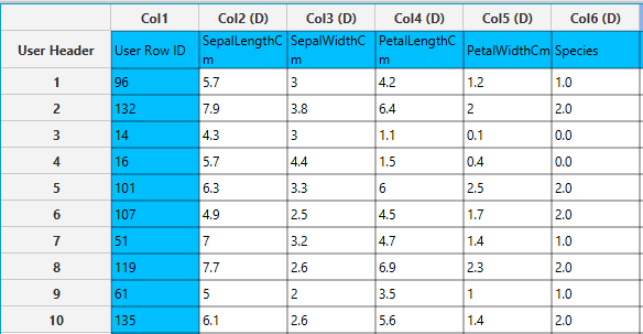
In the left-hand spreadsheet of the tab import the data matrix including the target variable for prediction. Note that the “Species” categorical column is presented as double (D).
Configuration
- Select
Analytics\(\rightarrow\)Regression\(\rightarrow\)Random Forest. - Specify the hyperparameters that determine the structure of the model: the
Features fraction[1],Min impurity decrease[2] andNumber of ensembles[4]. Default values, data types (double or integer) and acceptable ranges are indicated as guidance on the input parameter values. - Type a
Seedfor reproducible results or a random number generatedTime-based RNG Seed[3]. - Select the column name with the target variable that is going to be predicted from the drop-down menu [5].
- Click on the
Executebutton [6] to apply the training algorithm on the input columns

Output
In the right-hand spreadsheet of the tab the output data matrix with the actual and the predicted value of the target is presented.
Statistical fitting
MLR
Multiple Linear Regression is a statistical technique that predicts a dependent variable using two or more independent variables. MLR models the relationship between the dependent variable and the predictor using a linear equation. It is an extension of the simple linear regression allowing for more than one independent variable. An MLR model consists of the following key components:
- Mean Structure: The expected value of the response variable is modeled as a linear combination of predictors:
where \(\beta_0\) is the intercept, \(\beta_j\) are regression coefficients, \(x_{ij}\) are predictor values, and \(\epsilon_i\) is the error term.
- Assumptions: MLR relies on several key assumptions for valid inference:
- Linearity: The relationship between predictors and outcome is linear.
- Independence: Observations are independent of each other.
- Homoscedasticity: Errors have constant variance across all levels of predictors.
- Normality of errors: Residuals are normally distributed (for hypothesis testing).
- No multicollinearity: Predictors are not highly correlated with each other.
- Estimation Method: Coefficients are typically estimated using Ordinary Least Squares (OLS), which minimizes the sum of squared residuals.
- Interpretation of Coefficients: Each \(\beta_j\) represents the expected change in the dependent variable for a one-unit change in predictor , \(x_{ij}\), holding all other predictors constant.
- Model Evaluation: Goodness of fit and explanatory power are commonly assessed with metrics such as \(R^2\), adjusted \(R^2\), F-tests, and residual diagnostics.
This method is a simpler implementation allowing only for continuous data and main effects to be included in the model, if you want to perform multiple linear regression with categorical data and more complex options you can refer to Analytics \(\rightarrow\) Regression \(\rightarrow\) Statistical fitting \(\rightarrow\) Generalized Linear Models.
Use the MLR method by browsing in the top ribbon:
| Analytics \(\rightarrow\) Classification \(\rightarrow\) Statistical fitting \(\rightarrow\) MLR |
Input
The input should contain only numerical data and at least 2 columns should be specified, one corresponding to the target variable and at least 1 more to act as an independent predictor. All columns included in the input spreadsheet will be included in the analysis.
Configuration
| Target Column | Select from the drop-down menu the column containing the target variable that is going to be predicted. Columns with categorical features cannot be selected as targets. |
Output
A data matrix including the actual target value and the value predicted by the MLR method. Also the regression coefficients are present next to the predictions.
Example
Input
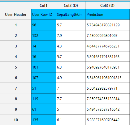
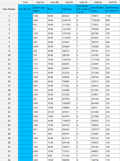
In the left-hand spreadsheet of the tab import the data matrix including the target variable for prediction.
Configuration
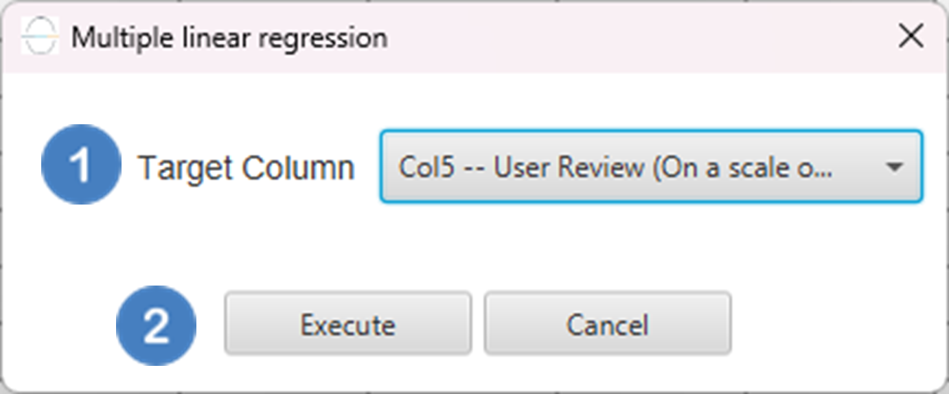
- Select
Analytics\(\rightarrow\)Classification\(\rightarrow\)Statistical fitting\(\rightarrow\)MLR. - Select the column that is going to be the
Target Column[1]. - Click on the
Executebutton [2] to apply the algorithm on the input table.
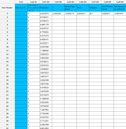
Output
In the right-hand spreadsheet of the tab the output data matrix with the actual and the predicted value of the target is presented. Also, the coefficients of the regression model are shown. The coefficient below “1” corresponds to the intercept and all other coefficients corresponds to the variable which has the name specified above the value.
Generalized Linear Models
Generalized Linear Models (GLMs) are a flexible class of regression models that generalize ordinary linear regression to allow for response variables that have error distributions other than the normal distribution. GLMs are particularly useful when the response variable is categorical (e.g., binary outcomes) or count data, where assumptions of normality and constant variance are inappropriate. A GLM consists of three components:
- Random Component: The response variable \(y_i\) is assumed to follow a distribution from the exponential family (e.g., Normal, Binomial, Poisson, Gamma).
- Systematic Component: A linear predictor \(\eta_i= x_i^T \beta\), where \(x_i\) is the vector of predictors for the i-th observation, and \(\beta\) is the vector of coefficients.
- Link Function: A smooth, monotonic function \(g(⋅)\) that relates the mean \(\mu_i= E[y_i]\) of the response to the linear predictor via \(g(\mu_i )= \eta_i\).
Unlike traditional linear regression, GLMs do not assume a linear relationship between the predictors and the response. Instead, the link function transforms the expected value of the response variable to a scale where it can be modeled as a linear combination of the predictors. GLM parameters are estimated using Maximum Likelihood Estimation (MLE). The likelihood is constructed based on the assumed distribution of the response variable, and the log-likelihood function is maximized to obtain the parameter estimates. Because log-likelihood is usually a nonlinear function of the parameters, iterative optimization method such as Newton-Raphson and Fisher Scoring are used to obtain the maximum likelihood estimates of the parameters of each model. Categorical variables are encoded using one-hot encoding, where each category is represented by a binary (0 or 1) dummy variable. The reference category for each categorical variable is the first observed category, and its corresponding dummy variable is omitted to avoid multicollinearity. This omission allows the reference category to be implicitly represented in the model intercept, providing a baseline for interpreting the effects of the other categories.
Linear
The classical linear regression model assumes that the response variable follows a normal (Gaussian) distribution, conditional on the explanatory variables. Specifically, for a continuous dependent variable \(Y\), the model expresses \(Y\) as a linear function of one or more independent variables \(X_1, X_2, …, X_p\), plus a normally distributed error term:
Within the framework of Generalized Linear Models (GLMs), linear regression corresponds to the case where the distribution of the dependent variable is Gaussian, and the link function is the identity function:
This identity link implies that the expected value of the outcome is directly modeled as a linear combination of the predictors. Linear regression is the most used when the dependent variable is continuous, unbounded, and approximately normally distributed, and when the relationship between the predictors and the outcome is assumed to be additive and linear.
Use the Linear Regression method by browsing in the top ribbon:
| Analytics \(\rightarrow\) Regression \(\rightarrow\) Statistical fitting \(\rightarrow\) Generalized Linear Models |
And then choosing “Linear” as the Type.
Input
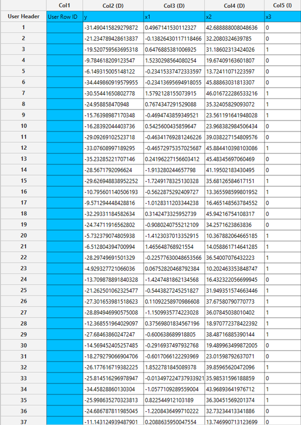
All variables need to be specified in the datasheet. Numerical values will be used for the covariates and the dependent variable. Factors, however, can be textual as well as numerical. The design for Linear Regression requires at least two columns in the input sheet: one column representing either a categorical factor or a covariate (independent variable), and another column for the numerical response. Each row represents a single observation.
Configuration
| Confidence Level (%) | Specify the confidence level of the analysis. Values should range from 0 to 100 and correspond to percentages. |
| Dependent Variable | Select the column that corresponds to values of the dependent variable. |
| Scale Parameter Method | Determines how the scale (error variance) parameter is estimated. Options include: Fixed value, Deviance, or Pearson Chi-square. |
| Value | Specifies the scale parameter value manually, only when Fixed value is selected in the Scale Parameter Method. |
| Factors/Covariates/Excluded Columns | Select manually the columns that correspond to factors and the columns that correspond to covariates through the dialog window: Use the buttons to move columns between the Factors and Covariates list and Excluded Columns list. Single-arrow buttons will move all selected columns and double-arrow buttons will move all columns. At least one covariate or factor column should be specified. |
| Specify Reference Levels | Specify the reference level for each of the categorical factors specified. The default option for each factor is its last level. |
| Formula Type | These options refer to the terms that will be included in the model. The Custom option allows the user to input a formula defining the exact terms to be included. The Main Effects option allows the analysis of a model that only includes all main effects and finally, the Full Factorial option includes both all main effects and all possible interaction terms to build a full model. |
| Specify Custom Model Formula | Specify the model formula used for the analysis if the Custom option is selected. The formula is created in the Custom Formula Creation dialog window by selecting factors and covariates and adding interaction terms up to the required order. Main effects of the included columns are always part of the model and cannot be excluded. |
Output
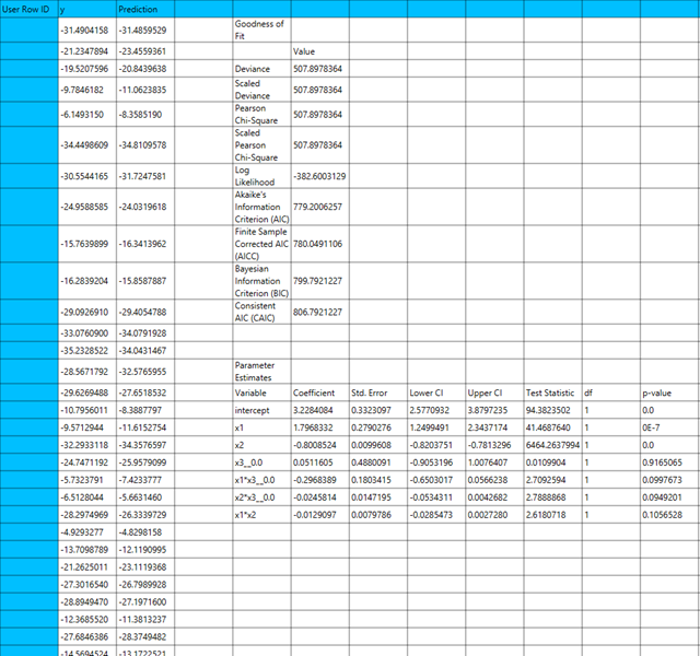
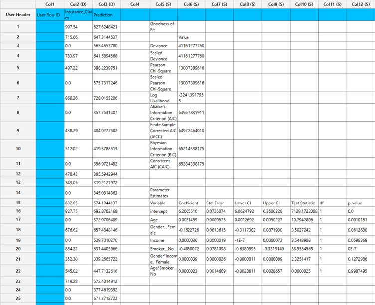
The output of the linear regression procedure is organized into:
- The Predicted Values Table contains the actual values of the dependent variable and the corresponding predicted values generated by the model for each observation.
- The Goodness of Fit Table includes statistical measures that assess how well the model fits the data, such as Deviance, Log-Likelihood, AIC, BIC, and related metrics.
- The Parameter Estimates Table displays the estimated coefficients for each variable in the model, along with standard errors, confidence intervals, test statistics, degrees of freedom, and p-values.
Example
Input
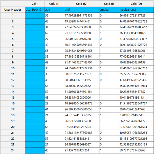
The input datasheet must include one continuous dependent variable, which will serve as the target, and at least one column with a continuous or categorical independent variable.
Configuration
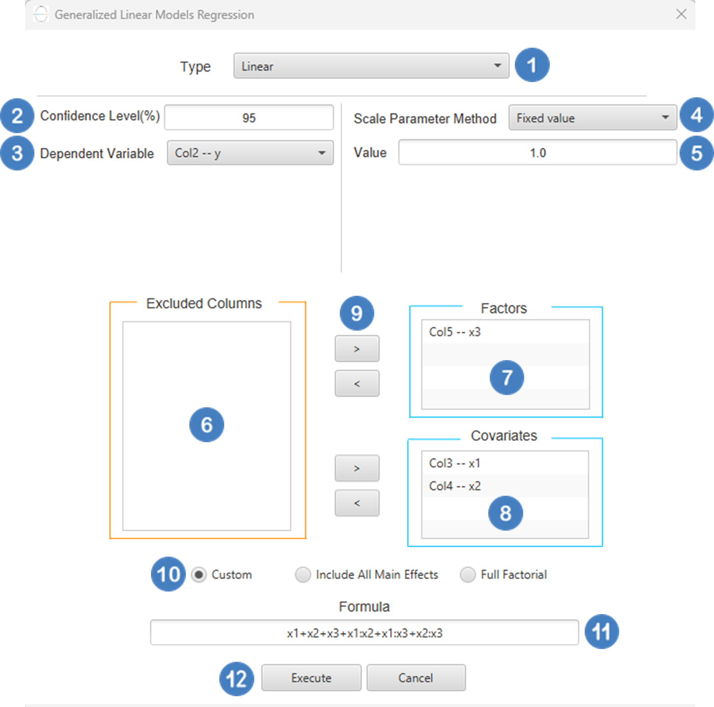
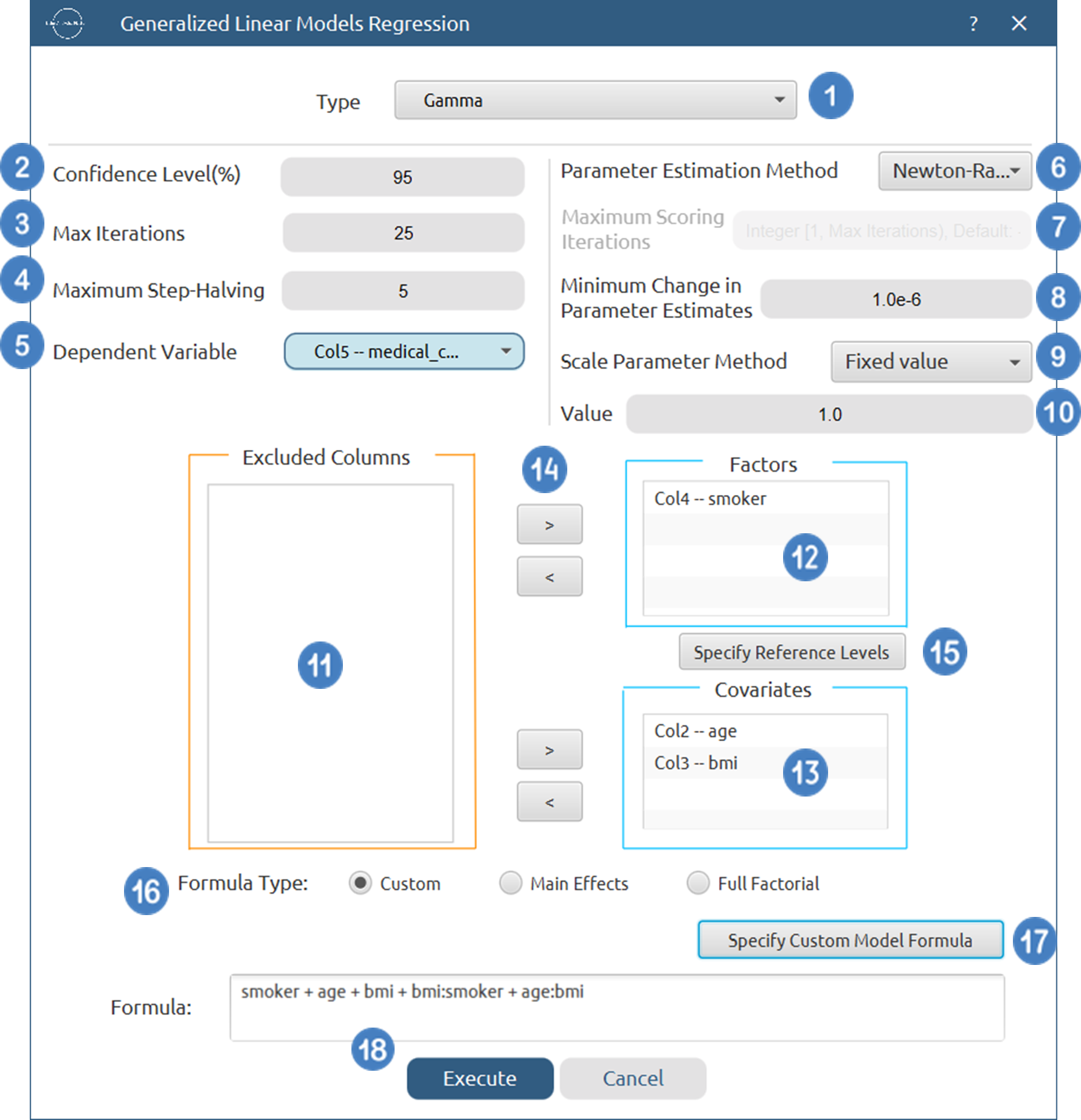
- Select
Analytics\(\rightarrow\)Regression\(\rightarrow\)Statistical fitting\(\rightarrow\)Generalized Linear Models - Set the
Type[1] of regression to Linear. - Specify the
Confidence Level (%)[2] for the test. - Select the
Dependent Variable[3]. - Select the
Scale Parameter Method[4]. - Specify the
Value[5] of the scale parameter method if the Fixed value option was chosen as the scale parameter method. - Select the columns by clicking on the arrow buttons [9] and moving columns between the
Excluded Columns[6] andFactors[7] andCovariates[8] lists. Specify Reference Levels[10] for the categorical factors.- Select the prefered
Formula Type[11]. Specify Custom Model Formula[12] for the analysis ifCustomoption is selected. How to specify a custom model formula?- Click on the
Executebutton [13] to perform the Linear Regression method.
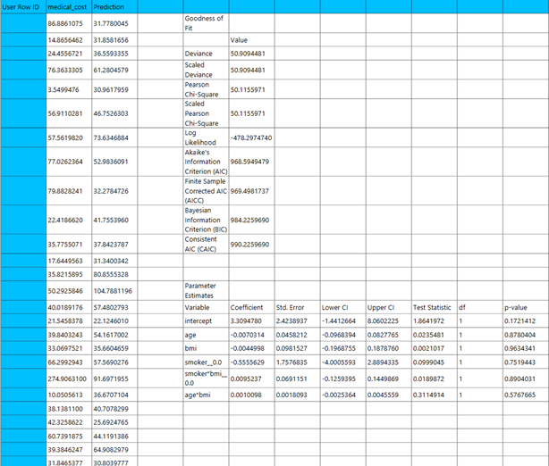
Output
The predictions, Goodness of Fit table and Parameter Estimates table are shown in the output spreadsheet.
Negative Binomial
Negative Binomial Regression is a type of generalized linear model (GLM) used for modeling count data that exhibit overdispersion – that is, when the variance exceeds the mean. It assumes that the dependent variable follows a Negative Binomial distribution, which is a generalization of the Poisson distribution that introduces an additional dispersion parameter to account for variability beyond the mean. The most commonly used link function is the log link, which models the logarithm of the expected count as a linear combination of the predictors:
Negative Binomial Regression is particularly useful in scenarios such as modeling the number of hospital visits, insurance claims, or any count-based outcome where the data are not well-fitted by Poisson model due to excess variation.
Use the Negative Binomial Regression method by browsing in the top ribbon:
| Analytics \(\rightarrow\) Regression \(\rightarrow\) Statistical fitting \(\rightarrow\) Generalized Linear Models |
And then choosing “Negative Binomial” as the Type.
Input
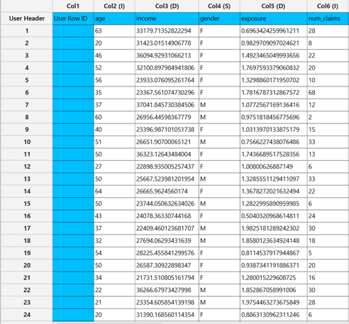
All variables must be specified in the datasheet. The dependent variable must be a non-negative integer count, as Negative Binomial Regression is designed for modeling count data. The dependent variable should not contain decimal values, negative numbers, or missing entries. Independent variables may be either numerical or categorical. Categorical variables can be represented using either text labels or numerical codes. The input datasheet must contain at least two columns: one for the dependent variable and one or more for the independent variables. Each row corresponds to single observation. This model is especially appropriate when the count data show overdispersion, meaning that the variance is greater than the mean – something that the standard Poisson model cannot adequately handle.
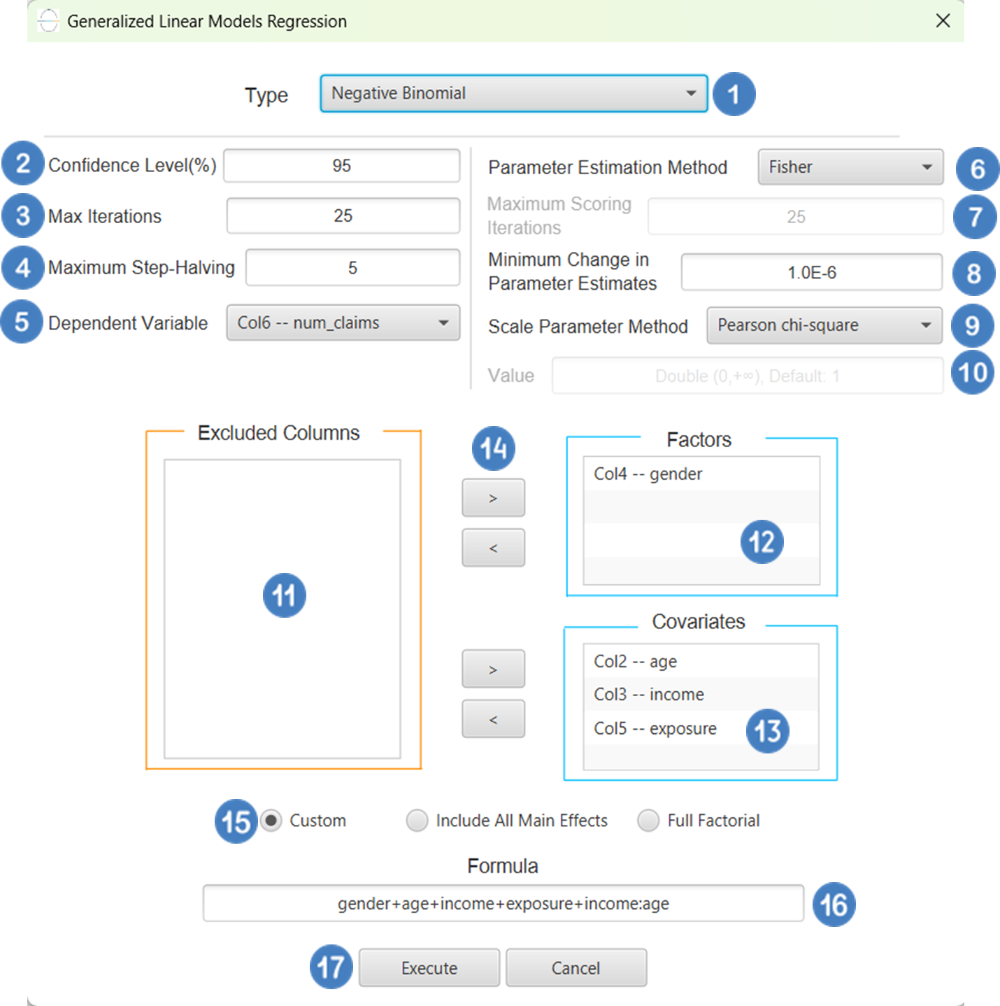
Configuration
| Confidence Level (%) | Specify the confidence level of the analysis. Values should range from 0 to 100 and correspond to percentages. |
| Max Iterations | Defines the maximum number of iterations the model is allowed to perform during the estimation process. If the model fails to converge before reaching this number, the algorithm stops and returns the values of the last iteration. |
| Maximum Step-Halving | Controls how many times the algorithm is allowed to halve the step size during parameter updates when an iteration leads to worse model fit. |
| Dependent Variable | Select the column that corresponds to values of the dependent variable. |
| Parameter Estimation | This option lets you choose how the model parameters will be estimated, Newton-Raphson, Fisher Scoring or Hybrid. |
| Maximum Scoring Iterations | The “Maximum Scoring Iterations” parameter is used when the hybrid estimation method is selected, instead of Newton-Raphson or Fisher scoring alone, and specifies the maximum number of iterations to be performed during the scoring phase. |
| Minimum Change in Parameter Estimates | Sets the tolerance level for convergence — the smallest change in parameter estimates between iterations required to continue optimization. If the change in all parameters is below this value, the algorithm assumes convergence has been reached. |
| Scale Parameter Method | Determines how the scale (error variance) parameter is estimated. Options include: Fixed value, Deviance, or Pearson Chi-square. |
| Value | Specifies the scale parameter value manually, only when Fixed value is selected in the Scale Parameter Method. |
| Factors/Covariates/Excluded Columns | Select manually the columns that correspond to factors and the columns that correspond to covariates through the dialog window: Use the buttons to move columns between the Factors and Covariates list and Excluded Columns list. Single-arrow buttons will move all selected columns and double-arrow buttons will move all columns. At least one covariate or factor column should be specified. |
| Specify Reference Levels | Specify the reference level for each of the categorical factors specified. The default option for each factor is its last level. |
| Formula Type | These options refer to the terms that will be included in the model. The Custom option allows the user to input a formula defining the exact terms to be included. The Main Effects option allows the analysis of a model that only includes all main effects and finally, the Full Factorial option includes both all main effects and all possible interaction terms to build a full model. |
| Specify Custom Model Formula | Specify the model formula used for the analysis if the Custom option is selected. The formula is created in the Custom Formula Creation dialog window by selecting factors and covariates and adding interaction terms up to the required order. Main effects of the included columns are always part of the model and cannot be excluded. |
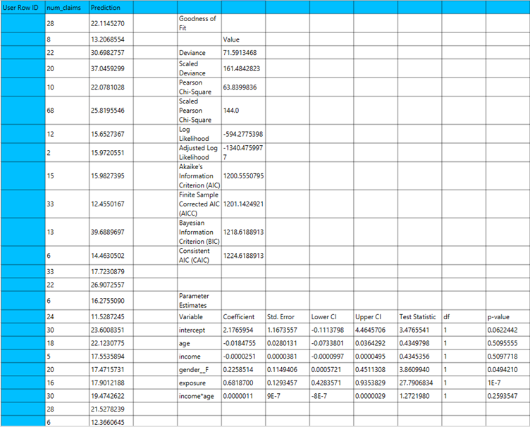
Output
The output of the Negative Binomial regression procedure is organized into three main sections: the Predicted Values Table, the Goodness of Fit Statistics, and the Parameter Estimates Table.
- The Predicted Values Table contains the actual values of the dependent variable and the corresponding predicted values generated by the model for each observation.
- The Goodness of Fit Table includes statistical measures that assess how well the model fits the data, such as Deviance, Log-Likelihood, AIC, BIC, and related metrics.
- The Parameter Estimates Table displays the estimated coefficients for each variable in the model, along with standard errors, confidence intervals, test statistics, degrees of freedom, and p-values.
Example
Input
The input datasheet must include one continuous, non-negative dependent variable, which will serve as the target, and at least one column with a continuous or categorical independent variable.
Configuration
- Select
Analytics\(\rightarrow\)Regression\(\rightarrow\)Statistical fitting\(\rightarrow\)Generalized Linear Models - Set the
Type[1] of regression to Negative Binomial. - Specify the
Confidence Level (%)[2] for the test. - Specify
Max Iterations[3]. - Specify the
Maximum Step-Halving[4]. - Select the
Dependent Variable[5]. - Select the
Parameter Estimation Method[6]. - Specify the
Maximum Scoring Iterationsif Hybrid option is selected as theParameter Estimation Method[7]. - Specify the
Minimum Change in Parameter Estimates[8]. - Select the
Scale Parameter Method[9]. - Specify the
Value[10] of the scale parameter method if the Fixed value option was chosen as the scale parameter method. - Select the columns by clicking on the arrow buttons [14] and moving columns between the
Excluded Columns[11] andFactors[12] andCovariates[13] lists. Specify Reference Levels[15] for the categorical factors.- Select the prefered
Formula Type[16]. Specify Custom Model Formula[17] for the analysis ifCustomoption is selected. How to specify a custom model formula?- Click on the
Executebutton [18] to perform the Negative Binomial Regression method.
Output
The predictions, Goodness of Fit table and Parameter Estimates table are shown in the output spreadsheet
Poisson
Poisson Regression is type of generalized linear model (GLM) used for modeling count data, where the dependent variable represents the number of times an event occurs within a fixed period, space, or exposure. It assumes that the response variable follows a Poisson distribution, where the mean is equal to the variance. The most common link function used is the log link, which relates the natural logarithm of the expected count to a linear combination of independent variables..
The independent variables can be either numerical or categorical, and they are used to explain variation in the count outcome. Poisson Regression is typically applied in cases such as modeling the number of doctor visits, traffic accidents, or product defects.
Use the Poisson Regression method by browsing in the top ribbon:
| Analytics \(\rightarrow\) Regression \(\rightarrow\) Statistical fitting \(\rightarrow\) Generalized Linear Models |
And then choosing “Poisson” as the Type.
Input
All variables must be specified in the datasheet. The dependent variable must be a non-negative integer count, as Poisson Regression is designed for modeling count data. The dependent variable should not contain decimal values, negative numbers, or missing entries. Independent variables may be either numerical or categorical. Categorical variables can be represented using either text labels or numerical codes. The input datasheet must include at least two columns: one for the dependent variable and one or more for the independent variables. Each row corresponds to a single observation. This model is appropriate when the count data has a variance approximately equal to the mean.
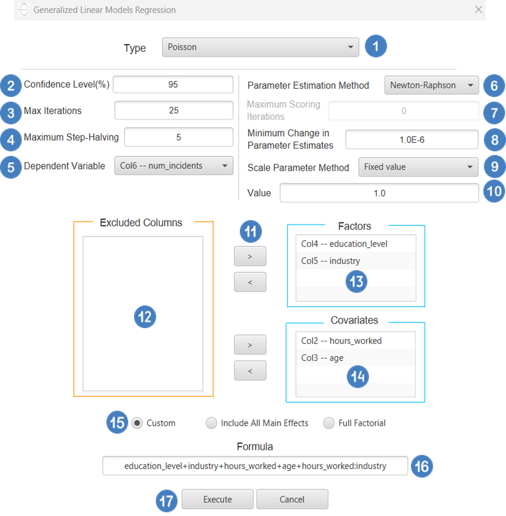
Configuration
| Confidence Level (%) | Specify the confidence level of the analysis. Values should range from 0 to 100 and correspond to percentages. |
| Max Iterations | Defines the maximum number of iterations the model is allowed to perform during the estimation process. If the model fails to converge before reaching this number, the algorithm stops and returns the values of the last iteration. |
| Maximum Step-Halving | Controls how many times the algorithm is allowed to halve the step size during parameter updates when an iteration leads to worse model fit. |
| Dependent Variable | Select the column that corresponds to values of the dependent variable. |
| Parameter Estimation | This option lets you choose how the model parameters will be estimated, Newton-Raphson, Fisher Scoring or Hybrid. |
| Maximum Scoring Iterations | The “Maximum Scoring Iterations” parameter is used when the hybrid estimation method is selected, instead of Newton-Raphson or Fisher scoring alone, and specifies the maximum number of iterations to be performed during the scoring phase. |
| Minimum Change in Parameter Estimates | Sets the tolerance level for convergence — the smallest change in parameter estimates between iterations required to continue optimization. If the change in all parameters is below this value, the algorithm assumes convergence has been reached. |
| Scale Parameter Method | Determines how the scale (error variance) parameter is estimated. Options include: Fixed value, Deviance, or Pearson Chi-square. |
| Value | Specifies the scale parameter value manually, only when Fixed value is selected in the Scale Parameter Method. |
| Factors/Covariates/Excluded Columns | Select manually the columns that correspond to factors and the columns that correspond to covariates through the dialog window: Use the buttons to move columns between the Factors and Covariates list and Excluded Columns list. Single-arrow buttons will move all selected columns and double-arrow buttons will move all columns. At least one covariate or factor column should be specified. |
| Specify Reference Levels | Specify the reference level for each of the categorical factors specified. The default option for each factor is its last level. |
| Formula Type | These options refer to the terms that will be included in the model. The Custom option allows the user to input a formula defining the exact terms to be included. The Main Effects option allows the analysis of a model that only includes all main effects and finally, the Full Factorial option includes both all main effects and all possible interaction terms to build a full model. |
| Specify Custom Model Formula | Specify the model formula used for the analysis if the Custom option is selected. The formula is created in the Custom Formula Creation dialog window by selecting factors and covariates and adding interaction terms up to the required order. Main effects of the included columns are always part of the model and cannot be excluded. |
Output
The output of the Poisson regression procedure is organized into three main sections: the Predicted Values Table, the Goodness of Fit Statistics, and the Parameter Estimates Table.
- The Predicted Values Table contains the actual values of the dependent variable and the corresponding predicted values generated by the model for each observation.
- The Goodness of Fit Table includes statistical measures that assess how well the model fits the data, such as Deviance, Log-Likelihood, AIC, BIC, and related metrics.
- The Parameter Estimates Table displays the estimated coefficients for each variable in the model, along with standard errors, confidence intervals, test statistics, degrees of freedom, and p-values.
Example
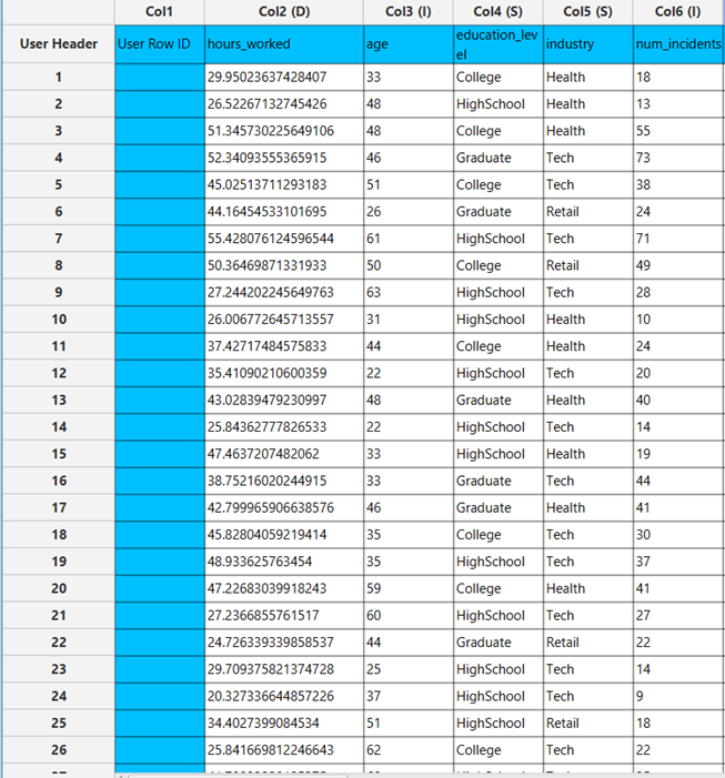
Input
Τhe dataset must include a target variable consisting of non-negative integer counts, appropriate for modeling with Poisson regression, and at least one column with a continuous or categorical independent variable.
Configuration
- Select
Analytics\(\rightarrow\)Regression\(\rightarrow\)Statistical fitting\(\rightarrow\)Generalized Linear Models - Set the
Type[1] of regression to Poisson. - Specify the
Confidence Level (%)[2] for the test. - Specify
Max Iterations[3]. - Specify the
Maximum Step-Halving[4]. - Select the
Dependent Variable[5]. - Select the
Parameter Estimation Method[6]. - Specify the
Maximum Scoring Iterationsif Hybrid option is selected as theParameter Estimation Method[7]. - Specify the
Minimum Change in Parameter Estimates[8]. - Select the
Scale Parameter Method[9]. - Specify the
Value[10] of the scale parameter method if the Fixed value option was chosen as the scale parameter method. - Select the columns by clicking on the arrow buttons [14] and moving columns between the
Excluded Columns[11] andFactors[12] andCovariates[13] lists. Specify Reference Levels[15] for the categorical factors.- Select the prefered
Formula Type[16]. Specify Custom Model Formula[17] for the analysis ifCustomoption is selected. How to specify a custom model formula?- Click on the
Executebutton [18] to perform the Poisson Regression method.
Output
The predictions, Goodness of Fit table and Parameter Estimates table are shown in the output spreadsheet.
Gamma with Identity Link
Gamma regression with Identity Link is a type of generalized linear model (GLM) used when the response variable is continuous, strictly positive, and right-skewed behavior. It assumes that the dependent variable follows a Gamma distribution, which is well-suited for modeling non-negative data with a variance that increases with the mean. The choice for the link function to be the identity link, relates the mean of the response variable to the linear predictors via the identity function.
Gamma regression is particularly useful in applications such as modeling costs, waiting times, insurance claims, or any scenario where the outcome is positive and skewed. It provides a flexible framework to account for heteroscedasticity and asymmetry in data.
Use the Gamma Regression with Identity Link method by browsing in the top ribbon:
| Analytics \(\rightarrow\) Regression \(\rightarrow\) Statistical fitting \(\rightarrow\) Generalized Linear Models |
And then choosing “Gamma with Identity Link” as the Type.
Input
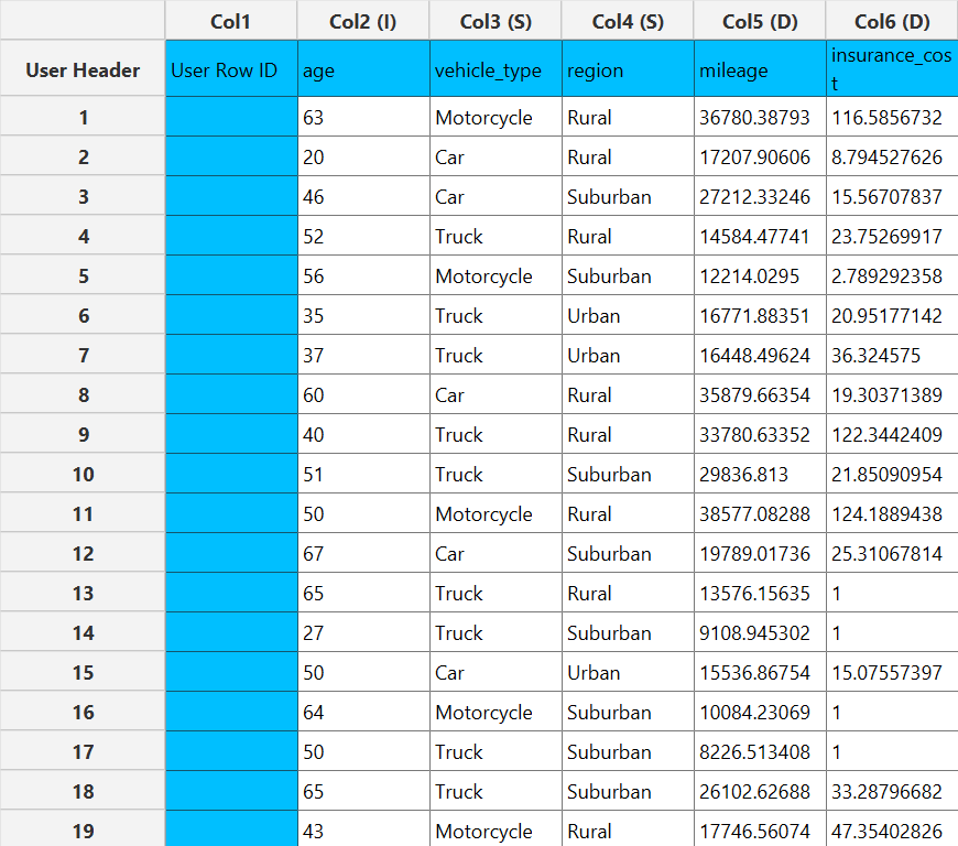
All variables must be specified in the datasheet. The dependent variable must be strictly positive continuous numerical variable, as Gamma regression is not defined for zero or negative values. Independent variables may be either numerical or numerical. Categorical factors can be represented as text labels or coded numerically. The input datasheet must include at least two columns: one for the dependent variable and one or more columns for the independent variables. Each row in the datasheet represents a single observation. It is important to check for zero or missing values in the dependent variable, as they may cause the model to fail or produce invalid estimates.
Configuration
| Confidence Level (%) | Specify the confidence level of the analysis. Values should range from 0 to 100 and correspond to percentages. |
| Max Iterations | Defines the maximum number of iterations the model is allowed to perform during the estimation process. If the model fails to converge before reaching this number, the algorithm stops and returns the values of the last iteration. |
| Maximum Step-Halving | Controls how many times the algorithm is allowed to halve the step size during parameter updates when an iteration leads to worse model fit. |
| Dependent Variable | Select the column that corresponds to values of the dependent variable. |
| Parameter Estimation | This option lets you choose how the model parameters will be estimated, Newton-Raphson, Fisher Scoring or Hybrid. |
| Maximum Scoring Iterations | The “Maximum Scoring Iterations” parameter is used when the hybrid estimation method is selected, instead of Newton-Raphson or Fisher scoring alone, and specifies the maximum number of iterations to be performed during the scoring phase. |
| Minimum Change in Parameter Estimates | Sets the tolerance level for convergence — the smallest change in parameter estimates between iterations required to continue optimization. If the change in all parameters is below this value, the algorithm assumes convergence has been reached. |
| Scale Parameter Method | Determines how the scale (error variance) parameter is estimated. Options include: Fixed value, Deviance, or Pearson Chi-square. |
| Value | Specifies the scale parameter value manually, only when Fixed value is selected in the Scale Parameter Method. |
| Factors/Covariates/Excluded Columns | Select manually the columns that correspond to factors and the columns that correspond to covariates through the dialog window: Use the buttons to move columns between the Factors and Covariates list and Excluded Columns list. Single-arrow buttons will move all selected columns and double-arrow buttons will move all columns. At least one covariate or factor column should be specified. |
| Specify Reference Levels | Specify the reference level for each of the categorical factors specified. The default option for each factor is its last level. |
| Formula Type | These options refer to the terms that will be included in the model. The Custom option allows the user to input a formula defining the exact terms to be included. The Main Effects option allows the analysis of a model that only includes all main effects and finally, the Full Factorial option includes both all main effects and all possible interaction terms to build a full model. |
| Specify Custom Model Formula | Specify the model formula used for the analysis if the Custom option is selected. The formula is created in the Custom Formula Creation dialog window by selecting factors and covariates and adding interaction terms up to the required order. Main effects of the included columns are always part of the model and cannot be excluded. |
Output
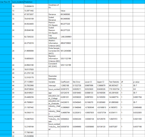
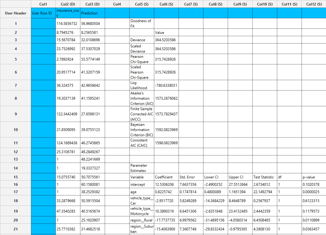
The output of the Gamma regression with Identity Link procedure is organized into three main sections: the Predicted Values Table, the Goodness of Fit Statistics, and the Parameter Estimates Table.
- The Predicted Values Table contains the actual values of the dependent variable and the corresponding predicted values 1. generated by the model for each observation.
- The Goodness of Fit Table includes statistical measures that assess how well the model fits the data, such as Deviance, Log-Likelihood, AIC, BIC, and related metrics.
- The Parameter Estimates Table displays the estimated coefficients for each variable in the model, along with standard errors, confidence intervals, test statistics, degrees of freedom, and p-values.
Example
Input
The input datasheet must include one continuous, positive dependent variable, which will serve as the target, and at least one column with a continuous or categorical independent variable.
Configuration
Configuration
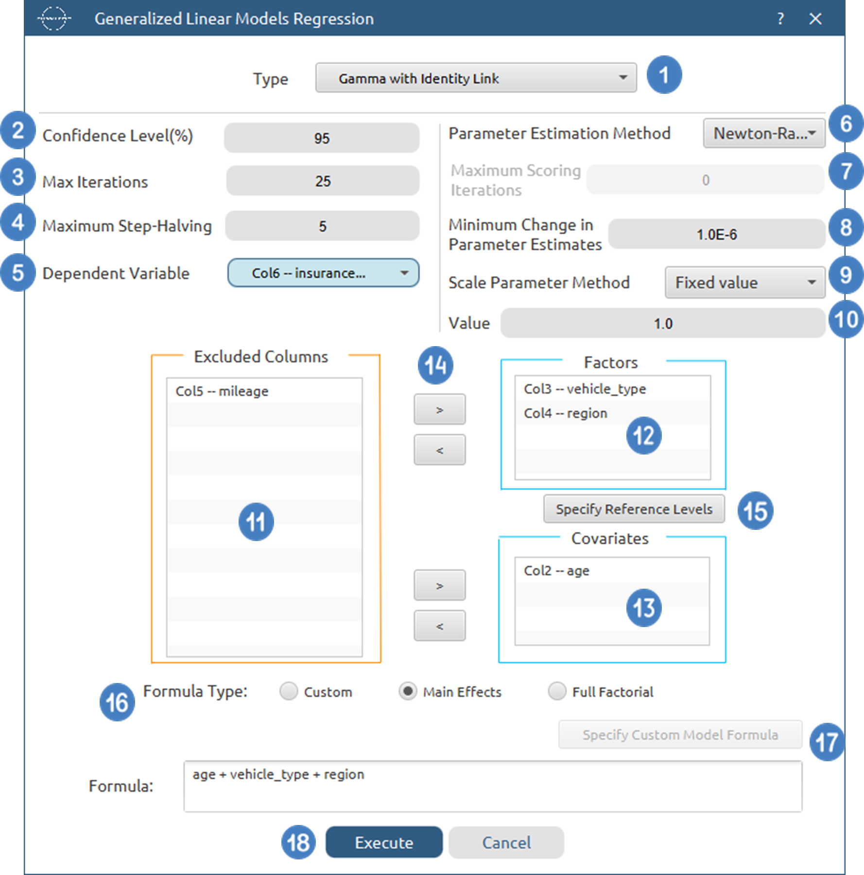
- Select
Analytics\(\rightarrow\)Regression\(\rightarrow\)Statistical fitting\(\rightarrow\)Generalized Linear Models - Set the
Type[1] of regression to Gamma with Identity Link. - Specify the
Confidence Level (%)[2] for the test. - Specify
Max Iterations[3]. - Specify the
Maximum Step-Halving[4]. - Select the
Dependent Variable[5]. - Select the
Parameter Estimation Method[6]. - Specify the
Maximum Scoring Iterationsif Hybrid option is selected as theParameter Estimation Method[7]. - Specify the
Minimum Change in Parameter Estimates[8]. - Select the
Scale Parameter Method[9]. - Specify the
Value[10] of the scale parameter method if the Fixed value option was chosen as the scale parameter method. - Select the columns by clicking on the arrow buttons [14] and moving columns between the
Excluded Columns[11] andFactors[12] andCovariates[13] lists. Specify Reference Levels[15] for the categorical factors.- Select the prefered
Formula Type[16]. Specify Custom Model Formula[17] for the analysis ifCustomoption is selected. How to specify a custom model formula?- Click on the
Executebutton [18] to perform the Gamma Regression with Identity Link method.
Output
The predictions, Goodness of Fit table and Parameter Estimates table are shown in the output spreadsheet.
Gamma with Log Link
Gamma regression with Log Link is a type of generalized linear model (GLM) used when the response variable is continuous, strictly positive, and right-skewed behavior. It assumes that the dependent variable follows a Gamma distribution, which is well-suited for modeling non-negative data with a variance that increases with the mean. The choice for the link function to be the log link, relates the mean of the response variable to the linear predictors via the natural logarithm.
Gamma regression is particularly useful in applications such as modeling costs, waiting times, insurance claims, or any scenario where the outcome is positive and skewed. It provides a flexible framework to account for heteroscedasticity and asymmetry in data.
Use the Gamma Regression with Log Link method by browsing in the top ribbon:
| Analytics \(\rightarrow\) Regression \(\rightarrow\) Statistical fitting \(\rightarrow\) Generalized Linear Models |
And then choosing “Gamma with Log Link” as the Type.
Input
All variables must be specified in the datasheet. The dependent variable must be strictly positive continuous numerical variable, as Gamma regression is not defined for zero or negative values. Independent variables may be either numerical or numerical. Categorical factors can be represented as text labels or coded numerically. The input datasheet must include at least two columns: one for the dependent variable and one or more columns for the independent variables. Each row in the datasheet represents a single observation. It is important to check for zero or missing values in the dependent variable, as they may cause the model to fail or produce invalid estimates.
Configuration
| Confidence Level (%) | Specify the confidence level of the analysis. Values should range from 0 to 100 and correspond to percentages. |
| Max Iterations | Defines the maximum number of iterations the model is allowed to perform during the estimation process. If the model fails to converge before reaching this number, the algorithm stops and returns the values of the last iteration. |
| Maximum Step-Halving | Controls how many times the algorithm is allowed to halve the step size during parameter updates when an iteration leads to worse model fit. |
| Dependent Variable | Select the column that corresponds to values of the dependent variable. |
| Parameter Estimation | This option lets you choose how the model parameters will be estimated, Newton-Raphson, Fisher Scoring or Hybrid. |
| Maximum Scoring Iterations | The “Maximum Scoring Iterations” parameter is used when the hybrid estimation method is selected, instead of Newton-Raphson or Fisher scoring alone, and specifies the maximum number of iterations to be performed during the scoring phase. |
| Minimum Change in Parameter Estimates | Sets the tolerance level for convergence — the smallest change in parameter estimates between iterations required to continue optimization. If the change in all parameters is below this value, the algorithm assumes convergence has been reached. |
| Scale Parameter Method | Determines how the scale (error variance) parameter is estimated. Options include: Fixed value, Deviance, or Pearson Chi-square. |
| Value | Specifies the scale parameter value manually, only when Fixed value is selected in the Scale Parameter Method. |
| Factors/Covariates/Excluded Columns | Select manually the columns that correspond to factors and the columns that correspond to covariates through the dialog window: Use the buttons to move columns between the Factors and Covariates list and Excluded Columns list. Single-arrow buttons will move all selected columns and double-arrow buttons will move all columns. At least one covariate or factor column should be specified. |
| Specify Reference Levels | Specify the reference level for each of the categorical factors specified. The default option for each factor is its last level. |
| Formula Type | These options refer to the terms that will be included in the model. The Custom option allows the user to input a formula defining the exact terms to be included. The Main Effects option allows the analysis of a model that only includes all main effects and finally, the Full Factorial option includes both all main effects and all possible interaction terms to build a full model. |
| Specify Custom Model Formula | Specify the model formula used for the analysis if the Custom option is selected. The formula is created in the Custom Formula Creation dialog window by selecting factors and covariates and adding interaction terms up to the required order. Main effects of the included columns are always part of the model and cannot be excluded. |
Output
The output of the Gamma regression with Log Link procedure is organized into three main sections: the Predicted Values Table, the Goodness of Fit Statistics, and the Parameter Estimates Table.
- The Predicted Values Table contains the actual values of the dependent variable and the corresponding predicted values 1. generated by the model for each observation.
- The Goodness of Fit Table includes statistical measures that assess how well the model fits the data, such as Deviance, Log-Likelihood, AIC, BIC, and related metrics.
- The Parameter Estimates Table displays the estimated coefficients for each variable in the model, along with standard errors, confidence intervals, test statistics, degrees of freedom, and p-values.
Example
Input
The input datasheet must include one continuous, positive dependent variable, which will serve as the target, and at least one column with a continuous or categorical independent variable.
Configuration
Configuration
- Select
Analytics\(\rightarrow\)Regression\(\rightarrow\)Statistical fitting\(\rightarrow\)Generalized Linear Models - Set the
Type[1] of regression to Gamma with Log Link. - Specify the
Confidence Level (%)[2] for the test. - Specify
Max Iterations[3]. - Specify the
Maximum Step-Halving[4]. - Select the
Dependent Variable[5]. - Select the
Parameter Estimation Method[6]. - Specify the
Maximum Scoring Iterationsif Hybrid option is selected as theParameter Estimation Method[7]. - Specify the
Minimum Change in Parameter Estimates[8]. - Select the
Scale Parameter Method[9]. - Specify the
Value[10] of the scale parameter method if the Fixed value option was chosen as the scale parameter method. - Select the columns by clicking on the arrow buttons [14] and moving columns between the
Excluded Columns[11] andFactors[12] andCovariates[13] lists. Specify Reference Levels[15] for the categorical factors.- Select the prefered
Formula Type[16]. Specify Custom Model Formula[17] for the analysis ifCustomoption is selected. How to specify a custom model formula?- Click on the
Executebutton [18] to perform the Gamma Regression with Log Link method.
Output
The predictions, Goodness of Fit table and Parameter Estimates table are shown in the output spreadsheet.
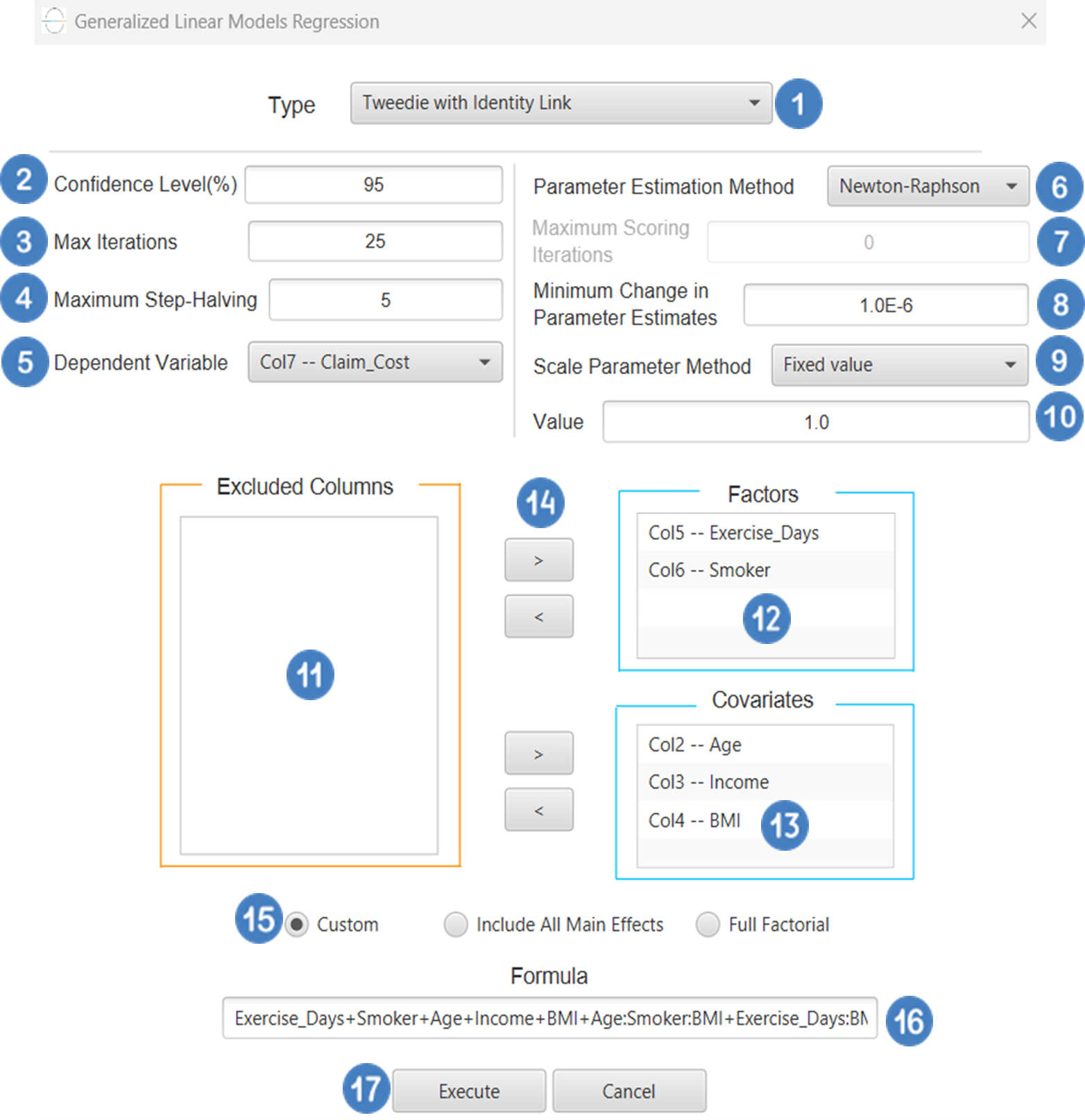
Tweedie with Identity Link
Tweedie Regression is a type of generalized linear model (GLM) designed to handle semi-continuous response variables, variables that exhibit a combination of many exact zeros and positive, continuous values. It assumes the response variable follows a Tweedie distribution, a member of the exponential dispersion family that encompasses distributions such as the normal, Poisson, gamma, and inverse Gaussian as special cases. When the Tweedie power parameter lies between 1 and 2, the distribution corresponds to a compound Poisson–Gamma process, which makes it particularly suitable for modeling zero-inflated, right-skewed data—such as insurance claim amounts, healthcare costs, or ecological measurements. In this formulation, the identity link function is used, meaning that the expected value of the response variable is modeled directly as a linear function of the predictors:
This link is appropriate when the response values are already on a meaningful scale and do not require transformation. However, care must be taken to ensure that the predicted values remain in a valid range (e.g., non-negative), since the identity link does not constrain the output.
Use the Tweedie Regression method with identity link by browsing in the top ribbon:
| Analytics \(\rightarrow\) Regression \(\rightarrow\) Statistical fitting \(\rightarrow\) Generalized Linear Models |
And then choosing “Tweedie with Identity Link” as the Type.
Input
All variables must be specified in the datasheet. The dependent variable must be a non-negative continuous numeric value, which may include many zeros alongside positive, right-skewed values. This reflects the typical structure of semi-continuous data for which Tweedie Regression with identity link is appropriate. Because the identity link function models the expected value directly, care should be taken to ensure that the response values are within a reasonable range, and that the model will not predict invalid (e.g., negative) values. The dependent variable should not contain negative numbers or missing entries. Independent variables may be either numerical or categorical. Categorical variables can be represented using text labels or numerical codes. The input datasheet must include at least two columns: one for the dependent variable and one or more for the independent variables. Each row should represent a single observation.
Configuration
| Confidence Level (%) | Specify the confidence level of the analysis. Values should range from 0 to 100 and correspond to percentages. |
| Max Iterations | Defines the maximum number of iterations the model is allowed to perform during the estimation process. If the model fails to converge before reaching this number, the algorithm stops and returns the values of the last iteration. |
| Maximum Step-Halving | Controls how many times the algorithm is allowed to halve the step size during parameter updates when an iteration leads to worse model fit. |
| Dependent Variable | Select the column that corresponds to values of the dependent variable. |
| Parameter Estimation | This option lets you choose how the model parameters will be estimated, Newton-Raphson, Fisher Scoring or Hybrid. |
| Maximum Scoring Iterations | The “Maximum Scoring Iterations” parameter is used when the hybrid estimation method is selected, instead of Newton-Raphson or Fisher scoring alone, and specifies the maximum number of iterations to be performed during the scoring phase. |
| Minimum Change in Parameter Estimates | Sets the tolerance level for convergence — the smallest change in parameter estimates between iterations required to continue optimization. If the change in all parameters is below this value, the algorithm assumes convergence has been reached. |
| Scale Parameter Method | Determines how the scale (error variance) parameter is estimated. Options include: Fixed value, Deviance, or Pearson Chi-square. |
| Value | Specifies the scale parameter value manually, only when Fixed value is selected in the Scale Parameter Method. |
| Factors/Covariates/Excluded Columns | Select manually the columns that correspond to factors and the columns that correspond to covariates through the dialog window: Use the buttons to move columns between the Factors and Covariates list and Excluded Columns list. Single-arrow buttons will move all selected columns and double-arrow buttons will move all columns. At least one covariate or factor column should be specified. |
| Specify Reference Levels | Specify the reference level for each of the categorical factors specified. The default option for each factor is its last level. |
| Formula Type | These options refer to the terms that will be included in the model. The Custom option allows the user to input a formula defining the exact terms to be included. The Main Effects option allows the analysis of a model that only includes all main effects and finally, the Full Factorial option includes both all main effects and all possible interaction terms to build a full model. |
| Specify Custom Model Formula | Specify the model formula used for the analysis if the Custom option is selected. The formula is created in the Custom Formula Creation dialog window by selecting factors and covariates and adding interaction terms up to the required order. Main effects of the included columns are always part of the model and cannot be excluded. |
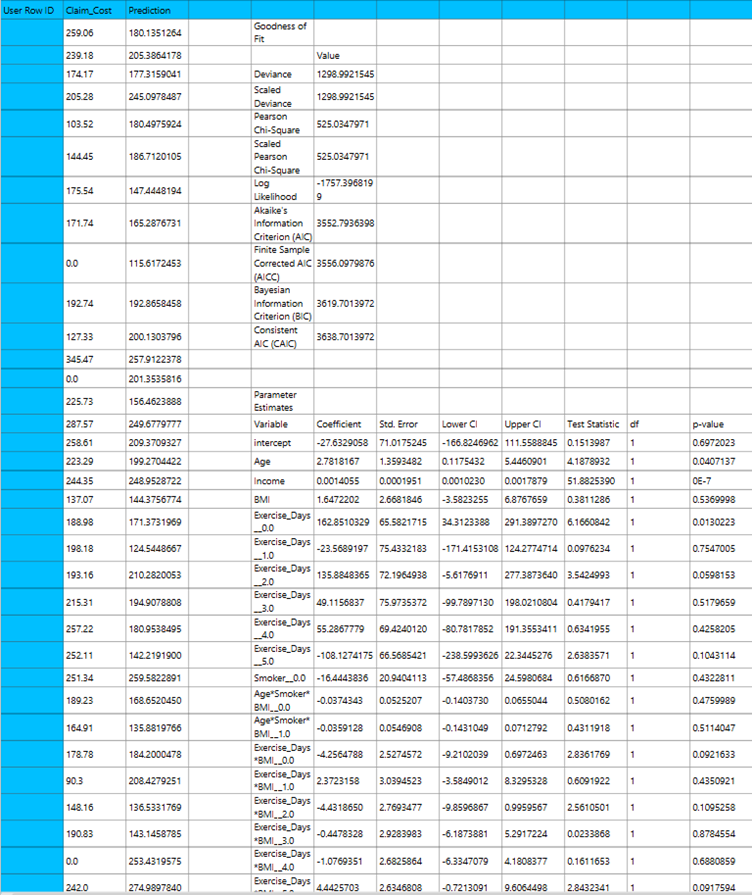
Output
The output of the Tweedie regression with identity link procedure is organized into three main sections: the Predicted Values Table, the Goodness of Fit Statistics, and the Parameter Estimates Table.
- The Predicted Values Table contains the actual values of the dependent variable and the corresponding predicted values generated by the model for each observation.
- The Goodness of Fit Table includes statistical measures that assess how well the model fits the data, such as Deviance, Log-Likelihood, AIC, BIC, and related metrics.
- The Parameter Estimates Table displays the estimated coefficients for each variable in the model, along with standard errors, confidence intervals, test statistics, degrees of freedom, and p-values.
Example
Input
The input datasheet must include one non-negative continuous dependent variable, which will serve as the target, and at least one column with a continuous or categorical independent variable.
Configuration
- Select
Analytics\(\rightarrow\)Regression\(\rightarrow\)Statistical fitting\(\rightarrow\)Generalized Linear Models - Set the
Type[1] of regression to Tweedie with Identity Link. - Specify the
Confidence Level (%)[2] for the test. - Specify
Max Iterations[3]. - Specify the
Maximum Step-Halving[4]. - Select the
Dependent Variable[5]. - Select the
Parameter Estimation Method[6]. - Specify the
Maximum Scoring Iterationsif Hybrid option is selected as theParameter Estimation Method[7]. - Specify the
Minimum Change in Parameter Estimates[8]. - Select the
Scale Parameter Method[9]. - Specify the
Value[10] of the scale parameter method if the Fixed value option was chosen as the scale parameter method. - Select the columns by clicking on the arrow buttons [14] and moving columns between the
Excluded Columns[11] andFactors[12] andCovariates[13] lists. Specify Reference Levels[15] for the categorical factors.- Select the prefered
Formula Type[16]. Specify Custom Model Formula[17] for the analysis ifCustomoption is selected. How to specify a custom model formula?- Click on the
Executebutton [18] to perform the Tweedie Regression with Identity Link method.
Output
The predictions, Goodness of Fit table and Parameter Estimates table are shown in the output spreadsheet.
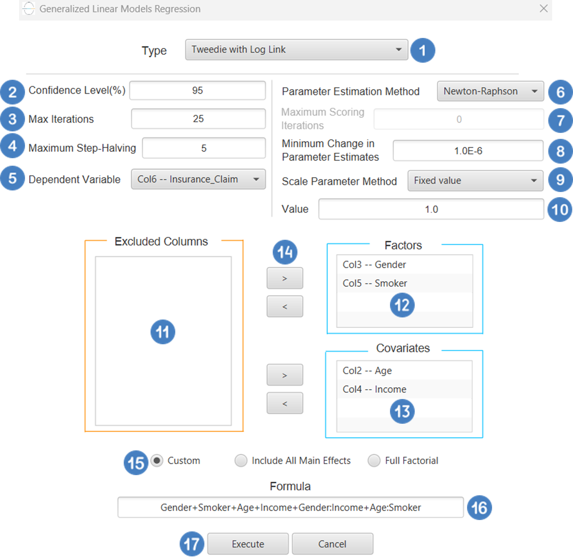
Tweedie with Log Link
Tweedie Regression is a type of generalized linear model (GLM) designed to handle semi-continuous response variables – that is, variables that take on many exact zeros and positive, continuous values otherwise. It assumes the response variable follows a Tweedie distribution, which belongs to the exponential dispersion family and includes the normal, Poisson, gamma and inverse Gaussian distributions as special cases. When the Tweedie power parameter lies between 1 and 2, the distribution corresponds to a compound Poisson- Gamma process, making it ideal for modeling zero-inflated, right-skewed data such as insurance claim amounts, healthcare expenditures, or ecological measurements. The most common link function used is the log link, where the logarithm of the expected value is modeled as a linear function of the predictors.
Use the Tweedie Regression with Log Link method by browsing in the top ribbon:
| Analytics \(\rightarrow\) Regression \(\rightarrow\) Statistical fitting \(\rightarrow\) Generalized Linear Models |
And then choosing “Tweedie with Log Link” as the Type.
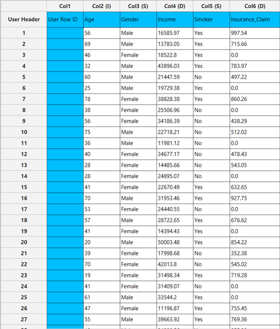
Input
All variables must be specified in the datasheet. The dependent variable must be a non-negative continuous numeric value, which may include many zeros alongside positive, right-skewed continuous values. This reflects the typical structure of semi-continuous data for which Tweedie Regression is appropriate. The dependent variable should not contain negative numbers or missing entries. Independent variables may be either numerical or categorical. Categorical variables can be represented using text labels or numerical codes. The input datasheet must include at least two columns: one for the dependent variable and one or more for the independent variables. Each row should represent a single observation.
Configuration
| Confidence Level (%) | Specify the confidence level of the analysis. Values should range from 0 to 100 and correspond to percentages. |
| Max Iterations | Defines the maximum number of iterations the model is allowed to perform during the estimation process. If the model fails to converge before reaching this number, the algorithm stops and returns the values of the last iteration. |
| Maximum Step-Halving | Controls how many times the algorithm is allowed to halve the step size during parameter updates when an iteration leads to worse model fit. |
| Dependent Variable | Select the column that corresponds to values of the dependent variable. |
| Parameter Estimation | This option lets you choose how the model parameters will be estimated, Newton-Raphson, Fisher Scoring or Hybrid. |
| Maximum Scoring Iterations | The “Maximum Scoring Iterations” parameter is used when the hybrid estimation method is selected, instead of Newton-Raphson or Fisher scoring alone, and specifies the maximum number of iterations to be performed during the scoring phase. |
| Minimum Change in Parameter Estimates | Sets the tolerance level for convergence — the smallest change in parameter estimates between iterations required to continue optimization. If the change in all parameters is below this value, the algorithm assumes convergence has been reached. |
| Scale Parameter Method | Determines how the scale (error variance) parameter is estimated. Options include: Fixed value, Deviance, or Pearson Chi-square. |
| Value | Specifies the scale parameter value manually, only when Fixed value is selected in the Scale Parameter Method. |
| Factors/Covariates/Excluded Columns | Select manually the columns that correspond to factors and the columns that correspond to covariates through the dialog window: Use the buttons to move columns between the Factors and Covariates list and Excluded Columns list. Single-arrow buttons will move all selected columns and double-arrow buttons will move all columns. At least one covariate or factor column should be specified. |
| Specify Reference Levels | Specify the reference level for each of the categorical factors specified. The default option for each factor is its last level. |
| Formula Type | These options refer to the terms that will be included in the model. The Custom option allows the user to input a formula defining the exact terms to be included. The Main Effects option allows the analysis of a model that only includes all main effects and finally, the Full Factorial option includes both all main effects and all possible interaction terms to build a full model. |
| Specify Custom Model Formula | Specify the model formula used for the analysis if the Custom option is selected. The formula is created in the Custom Formula Creation dialog window by selecting factors and covariates and adding interaction terms up to the required order. Main effects of the included columns are always part of the model and cannot be excluded. |
Output
The output of the Tweedie regression with log link procedure is organized into three main sections: the Predicted Values Table, the Goodness of Fit Statistics, and the Parameter Estimates Table.
- The Predicted Values Table contains the actual values of the dependent variable and the corresponding predicted values generated by the model for each observation.
- he Goodness of Fit Table includes statistical measures that assess how well the model fits the data, such as Deviance, Log-Likelihood, AIC, BIC, and related metrics.
- The Parameter Estimates Table displays the estimated coefficients for each variable in the model, along with standard errors, confidence intervals, test statistics, degrees of freedom, and p-values.
Example
Input
The input datasheet must include one non-negative continuous dependent variable, which will serve as the target, and at least one column with a continuous or categorical independent variable.
Configuration
- Select
Analytics\(\rightarrow\)Regression\(\rightarrow\)Statistical fitting\(\rightarrow\)Generalized Linear Models - Set the
Type[1] of regression to Tweedie with Log Link. - Specify the
Confidence Level (%)[2] for the test. - Specify
Max Iterations[3]. - Specify the
Maximum Step-Halving[4]. - Select the
Dependent Variable[5]. - Select the
Parameter Estimation Method[6]. - Specify the
Maximum Scoring Iterationsif Hybrid option is selected as theParameter Estimation Method[7]. - Specify the
Minimum Change in Parameter Estimates[8]. - Select the
Scale Parameter Method[9]. - Specify the
Value[10] of the scale parameter method if the Fixed value option was chosen as the scale parameter method. - Select the columns by clicking on the arrow buttons [14] and moving columns between the
Excluded Columns[11] andFactors[12] andCovariates[13] lists. Specify Reference Levels[15] for the categorical factors.- Select the prefered
Formula Type[16]. Specify Custom Model Formula[17] for the analysis ifCustomoption is selected. How to specify a custom model formula?- Click on the
Executebutton [18] to perform the Tweedie Regression with Log Link method.
Output
The predictions, Goodness of Fit table and Parameter Estimates table are shown in the output spreadsheet.
Loglinear Models
Log-linear models are a special case of generalized linear models that explain how cell counts vary across the levels of categorical variables in a contingency table. They also let us examine associations and interaction patterns among those variables. By default, these models treat the predictors (factors) as nominal, and the response is the count for each combination of factor levels—either the implicit number of times a combination appears in the raw data or, when present, the value in a frequency column.
In practice, they fit a GLM with a logarithmic link function and a Poisson or a Multinomial distribution for the response variable, estimating:
where \(\mu\) is the expected count for a given set of factor levels. The \(x_s\) are indicator variables for factor levels and their interactions.
A saturated log-linear model includes all main effects and all possible interactions among the factors. It exactly reproduces the observed cell counts, so the fitted means, \(\hat{\mu_i}\), equal the data, \(y_i\), the residual deviance is 0, and the residual degrees of freedom are 0. Because diagnostics like standardized/adjusted residuals can involve divisions by \(\sqrt{\hat{\mu_i}}\), we optionally add a small positive constant \(\delta\) when the model is saturated to avoid division by zero when \(𝑦_𝑖=0\).
Beyond the saturated case, there is also a custom model option where we include only the terms we want (e.g., main effects only, selected two-way interactions, etc.).
For each cell (factor combination) we provide the following cell diagnostics:
- Observed count: $$ \begin{equation} y_i \end{equation} $$
- Observed percentage: $$ \begin{equation} \frac{y_i}{\sum_{i=1}^n y_i} \end{equation} $$
- Expected count $$ \begin{equation} \hat{\mu_i} \end{equation} $$
- Expected percentage: $$ \begin{equation} \frac{\hat{\mu_i}}{\sum_{i=1}^n \hat{\mu_i}} \end{equation} $$
- Residual: $$ \begin{equation} r_i = y_i - \hat{\mu_i} \end{equation} $$
- Standardized Residual: $$ \begin{equation} r_i^{std} = \frac{y_i - \hat{\mu_i}}{\sqrt{\hat{\mu_i}}} \end{equation} $$
- Adjusted Residual: $$ \begin{equation} r_i^{adj} = \frac{y_i - \hat{\mu_i}}{\sqrt{\hat{\mu_i}}(1-h_{ii})} \end{equation} $$
where \(h_{ii}\) is the i-th diagonal element of the hat matrix.
- Deviance Residual: $$ \begin{equation} d_i = 2sign(y_i-\hat{\mu_i})[y_ilog(\frac{y_i}{\hat{\mu_i}}) - (y_i \hat{\mu_i})] \end{equation} $$
Use the Loglinear Model method by browsing in the top ribbon:
| Analytics \(\rightarrow\) Regression \(\rightarrow\) Statistical fitting \(\rightarrow\) Loglinear Models |
Input
All variables need to be specified in the data sheet. Numerical values will be used for the cell covariates as well as for dependent variables, which is the cell count or frequency. Factors, however, can be textual as well as numerical. The design for log-linear modeling requires at least two elements in the input sheet: one or more columns representing the categorical factors that define the contingency cells, and either a numeric frequency column (for pre-aggregated tables) or raw rows with no frequency column (in which case counts are computed from the repetitions). Each row represents a single observation in the raw-data case and corresponds to a single cell in the aggregated-table case; optional cell covariates can be included as additional numeric columns.
Configuration
| Distribution of Cell Counts | Specify the desired distribution of cell counts. Available options include Poisson and Multinomial. |
| Confidence Level(%) | Specify the confidence level of the analysis. Values should range from 0 to 100 and correspond to percentages. |
| Max Iterations | Defines the maximum number of iterations the model is allowed to perform during the estimation process. If the model fails to converge before reaching this number, the algorithm stops and returns the values of the last iteration. |
| Minimum Change in Parameter Estimates | Sets the tolerance level for convergence — the smallest change in parameter estimates between iterations required to continue optimization. If the change in all parameters is below this value, the algorithm assumes convergence has been reached. |
| Delta | Specify a small positive constant added only for numerical stability when the model is saturated (perfect fit). Values should range from 0 to 1 with the default option being 0.5. |
| Do not weight cases/ Weight cases by | Choose whether each row contributes equally or according to a weight variable. If the “Do not weight cases” option is selected, then each row counts as 1. If the “Weight cases by” option is selected, select a numeric column to be treated as the frequency. For each factor combination, the model uses the sum of that column as the cell frequency. Values must be numerical and non-negative. |
| Factors/Cell Covariates/Excluded Columns | Select manually the columns that correspond to factors and the columns that correspond to cell covariates through the dialog window: Use the buttons to move columns between the Factors and Cell Covariates list and Excluded Columns list. Single-arrow buttons will move all selected columns and double-arrow buttons will move all columns. At least one factor column should be specified. |
| Specify Reference Levels | Specify the reference level for each of the categorical factors specified. The default option for each factor is its last level. |
| Formula Type | These options refer to the terms that will be included in the model. The Custom option allows the user to input a formula defining the exact terms to be included. The Saturated Model option includes both all main effects and all possible interaction terms to build a full model.Note that the Saturated Model option does not allow the use of a formula. |
| Specify Custom Model Formula | Specify the model formula used for the analysis if the Custom option is selected. The formula is created in the Custom Formula Creation dialog window by selecting factors and covariates and adding interaction terms up to the required order. Main effects of the included columns are always part of the model and cannot be excluded. |
Output
The output of the log-linear procedure is organized into four sections: the Counts & Residuals Table, the Covariance Matrix, the Correlations Matrix and the Parameter Estimates Table. The Counts & Residuals Table provides the cell diagnostics we discussed earlier. For each cell we provide the Observed count, the Observed percentage, the Expected Count, The Expected Percentage, the Residual, the Standardized Residual, the Adjusted Residual and the Deviance. The Covariance and Correlations matrices show the covariance and correlation of each pair of variables in the model accordingly. The Parameter Estimates Table displays the estimated coefficients for each variable in the model, along with standard errors, confidence intervals, test statistics, degrees of freedom, and p-values.
Example
Input
The input datasheet must include at least one factor variable, either numeric or textual.
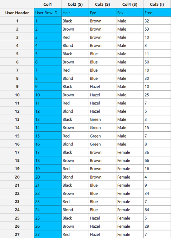
Configuration
- Select
Analytics\(\rightarrow\)Regression\(\rightarrow\)Statistical fitting\(\rightarrow\)Loglinear Models. - Select the
Distribution of Cell Counts[1]. - Specify the
Confidence Level (%)[2] for the test. - Specify
Max Iterations[3]. - Specify the
Minimum Change in Parameter Estimates[4]. - Specify the
Delta[5] parameter for numerical stability. - Choose whether to
Do not weight casesorWeight cases by[6]. If theWeight cases byoption is selected, specify thefrequencycolumn[7]. - Select the columns by clicking on the arrow buttons [11] and moving columns between the
Excluded Columns[8] andFactors[9] andCell Covariates[10] lists. Specify Reference Levels[12] for the categorical factors.- Select the prefered
Formula Type[13]. Specify Custom Model Formula[14] for the analysis ifCustomoption is selected. How to specify a custom model formula?- Click on the
Executebutton [15] to perform the Loglinear method.
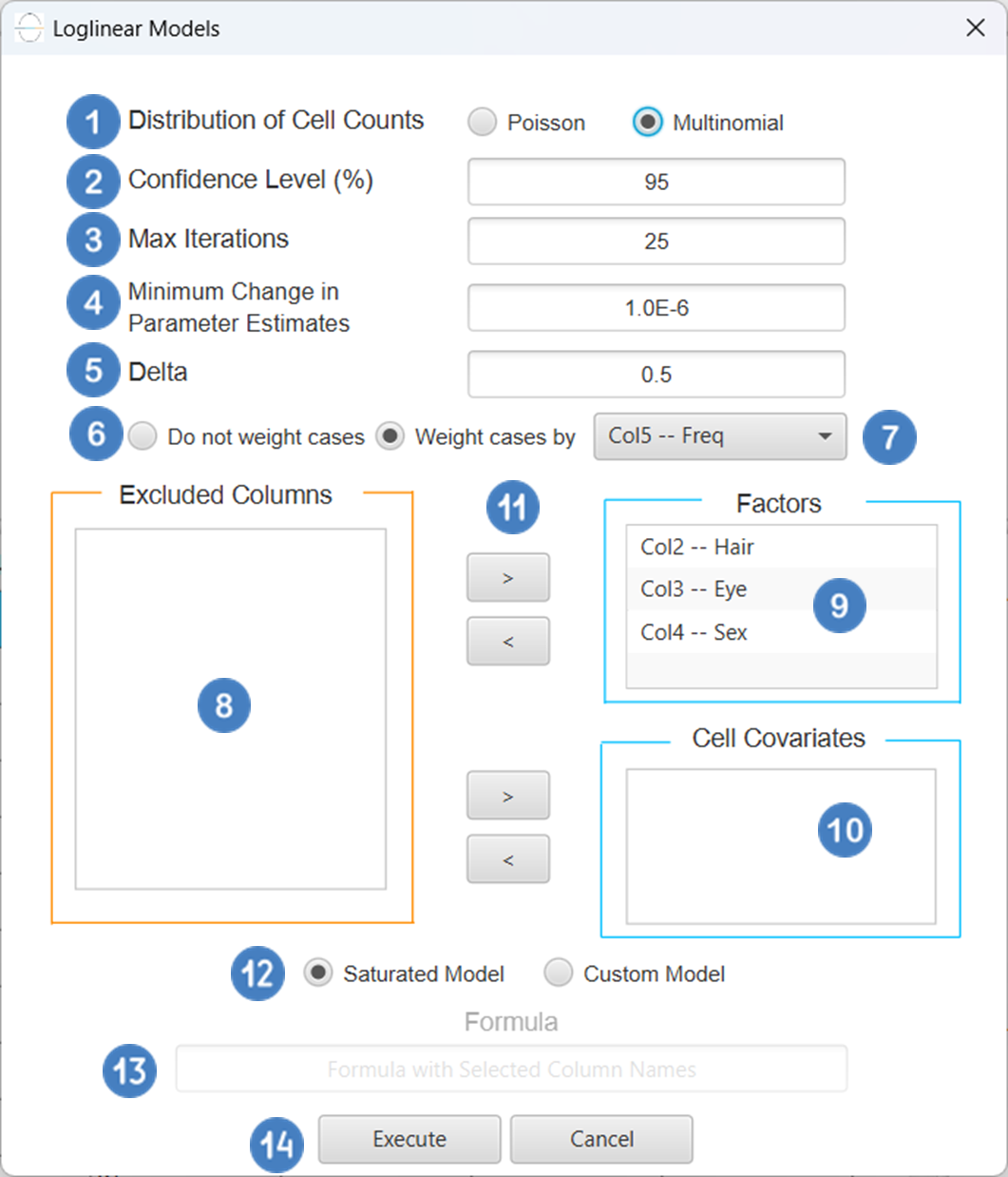
Output
The Counts & Residuals Table, Covariance Matrix, Correlations Matrix and the Parameter Estimates Table are shown in the output spreadsheet.
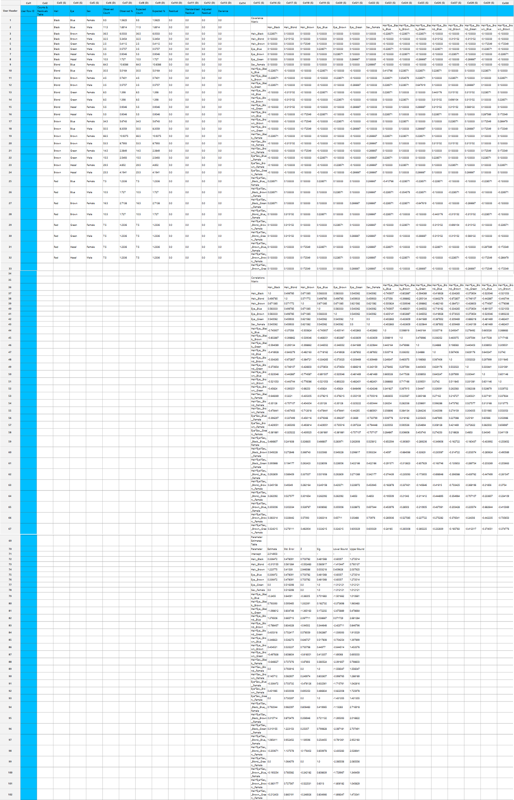
Generalized Estimating Equations
Generalized Estimating Equations (GEEs) extend Generalized Linear Models (GLMs) to handle correlated or clustered response data, such as repeated measures or longitudinal observations. GEEs are particularly useful when responses are not independent, as they allow for within-subject correlation, making them ideal for analyzing data collected over time or across related units. A GEE model consists of the following key components:
- Mean Structure: Like GLMs, the expected value of the response variable is modeled using a linear predictor :
Where \(x_i\) is the vector of predictors and \(\beta\) is the vector of coefficients.
- Link Function: A monotonic function \(g(∙)\) that links the mean of the response \(\mu_i= E[y_i]\) to the linear predictor, so that \(g(\mu_i)=\eta_i\).
- Working Correlation Matrix: Specifies the assumed correlation structure among repeated observations within the same subject. Common structures include:
- Independent: assumes no within-subject correlation.
- Exchangeable: assumes equal correlation between all pairs of observations.
- AR(1): assumes correlations decrease with time distance.
- Unstructured: allows a distinct correlation for each pair of observations, with no constraints.
- M-dependent: assumes nonzero correlations only up to lag M, and zero correlations beyond that distance.
GEE estimation relies on solving quasi-likelihood equations rather than maximizing a full likelihood function, making it a semi-parametric approach. Parameters are estimated using iterative methods such as iteratively reweighted least squares (IRLS), and standard errors are typically computed using robust estimators to ensure valid inference even if the correlation structure is misspecified. In GEE models, a subject variable is required to identify the unit over which repeated measurements occur (e.g., patient ID). Optionally, a within-subject variable (e.g., time or visit number) can be specified to define the ordering of repeated measurements. Cases are usually sorted by subject and within-subject variables to ensure correct modeling of correlation patterns. The robust covariance estimator is the default choice, providing consistent standard errors under mild assumptions. The model-based estimator may be more efficient if the correlation structure is correctly specified, but it is more sensitive to misspecification. Categorical variables are encoded using dummy coding, as in GLMs. The reference category is omitted by default to avoid multicollinearity and serve as a baseline for interpreting effects.
Each variant of this method is specified by the distribution of the response variable and the link function used. In the table below we specify the distribution and link function used for each variant:
| GEE Variant | Distribution | Link Function |
| Linear | Normal | Identity |
| Negative Binomial | Negative Binomial | Log |
| Poisson | Poisson | Log |
| Gamma | Gamma | Log |
| Tweedie with Identity Link | Tweedie | Identity |
| Tweedie with Log Link | Tweedie | Log |
Linear
Use the Linear Regression method by browsing in the top ribbon:
| Analytics \(\rightarrow\) Regression \(\rightarrow\) Statistical fitting \(\rightarrow\) Generalized Estimating Equations |
And then choosing “Linear” as the Type.
Input
All variables must be specified in the datasheet. The dependent variable must be numerical, as Linear Regression within the GEE framework models continuous outcomes. Covariates should also be numerical, while categorical predictors (factors) can be represented using either text labels or numeric codes. The input datasheet must include at least two columns: one for the dependent variable and one or more for the independent variables (covariates or factors). Each row should correspond to a single observation. Additionally, a subject identifier column is required to define clusters of repeated measurements, and optionally a within-subject variable (e.g., time) to specify the order of observations within each subject.
Configuration
| Confidence Level (%) | Specify the confidence level of the analysis. Values should range from 0 to 100 and correspond to percentages. |
| Max Iterations | Defines the maximum number of iterations the model is allowed to perform during the estimation process. If the model fails to converge before reaching this number, the algorithm stops and returns the values of the last iteration. |
| Iterations Between Updates | Defines how often the working correlation matrix is updated during estimation. |
| Dependent Variable | Select the column that corresponds to values of the dependent variable. |
| Minimum Change in Parameter Estimates | Sets the tolerance level for convergence — the smallest change in parameter estimates between iterations required to continue optimization. If the change in all parameters is below this value, the algorithm assumes convergence has been reached. |
| Hessian Convergence | Specifies a threshold for convergence based on the second derivatives (Hessian matrix). |
| Scale Parameter | Adjusts the variance of the model. |
| Within Subject | Selects the column that defines the ordering of repeated observations within each subject. |
| Structure | Defines the working correlation structure for repeated measurements within subjects. Choices include Independent, Exchangeable, AR(1), Unstructured and M-Dependent. |
| M | In the M-Dependent correlation structure, M specifies the maximum number of consecutive observations within each cluster that are assumed to be correlated, with correlations set to zero for observations more than M time points apart. M must be an integer in the range from 1 to (number of within-subject observations – 1). |
| Covariance Matrix | In the Covariance Matrix option, the user selects how the model’s standard errors will be estimated. The Robust estimator is resistant to misspecification of the correlation structure, while the Model-based estimator assumes the specified correlation is correct. |
| Subjects/Factors/Covariates/Excluded Columns | Select manually the columns that correspond to subjects, factors and the columns that correspond to covariates through the dialog window: Use the buttons to move columns between the Subjects, Factors and Covariates list and Excluded Columns list. Single-arrow buttons will move all selected columns. At least one covariate or factor column should be specified. Also, a column for the Subject is required. |
| Specify Reference Levels | Specify the reference level for each of the categorical factors specified. The default option for each factor is its last level. |
| Formula Type | These options refer to the terms that will be included in the model. The Custom option allows the user to input a formula defining the exact terms to be included. The Main Effects option allows the analysis of a model that only includes all main effects and finally, the Full Factorial option includes both all main effects and all possible interaction terms to build a full model. |
| Specify Custom Model Formula | Specify the model formula used for the analysis if the Custom option is selected. The formula is created in the Custom Formula Creation dialog window by selecting factors and covariates and adding interaction terms up to the required order. Main effects of the included columns are always part of the model and cannot be excluded. |
Output
The output of the Generalized Estimating Equations (GEEs) procedure is organized into three main sections: the Predicted Values Table, the Parameter Estimates Table and the Working Correlation Matrix.
- The Predicted Values Table shows the fitted values for the dependent variable on the specified model.
- The Parameter Estimates Table includes the estimated coefficients for the independent variables. Each row corresponds to a predictor and includes its coefficient, standard error, confidence interval, test statistic, degrees of freedom, and p-value.
- The Working Correlation Matrix displays the estimated correlations between repeated measurements of the same subject over time.
Example
Input
The dataset must include a continuous target variable suitable for modeling with linear regression. It should also contain at least one independent variable, which can be continuous or categorical. In addition, the dataset must include a subject identifier to group repeated observations from the same individual or unit, as well as a within-subject time or measurement indicator to reflect the longitudinal or clustered nature of the data.
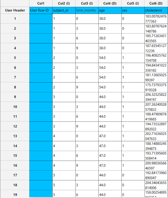
Configuration
- Select
Analytics\(\rightarrow\)Regression\(\rightarrow\)Statistical fitting\(\rightarrow\)Generalized Estimating Equations. - Set the
Type[1] of regression to Linear. - Specify the
Confidence Level (%)[2] for the test. - Specify
Max Iterations[3]. - Specify
Iterations Between Updates[4]. - Select the
Dependent Variable[5]. - Specify the
Minimum Change in Parameter Estimates[6]. - Specify the
Hessian Convergence[7]. - Specify the
Scale Parameter[8]. - Select the
Within Subject[9]. - Select the
working correlation Structureand specify the value ofMif you select M-Dependent as the correlation structure. [10]. - Select the method used to estimate the
covariance matrix[11] of the standard errors. - Select the columns by clicking on the arrow buttons [16] and moving columns between the
Excluded Columns[12] andSubjects[13] andFactors[14] andCovariates[15] lists. Specify Reference Levels[17] for the categorical factors.- Select the prefered
Formula Type[18]. Specify Custom Model Formula[19] for the analysis ifCustomoption is selected. How to specify a custom model formula?- Click on the
Executebutton [20] to perform the Linear Regression method.
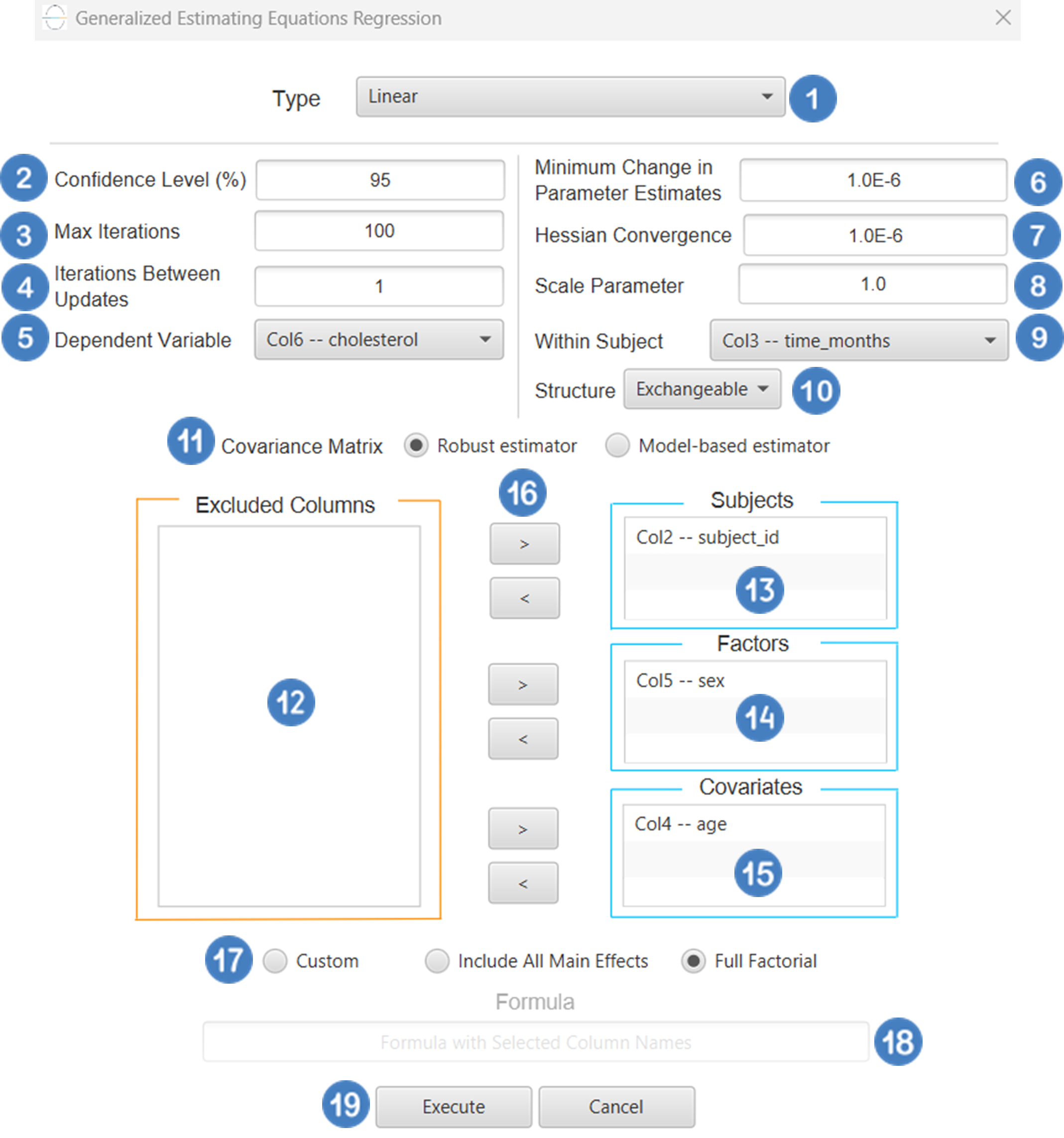
Output
The Predictions, Parameter Estimates table and Working Correlation Matrix are shown in the output spreadsheet.
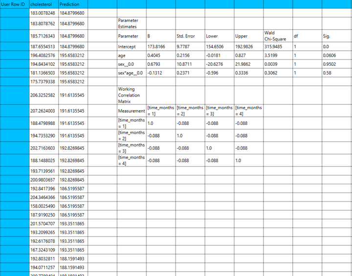
Negative Binomial
Use the Negative Binomial Regression method by browsing in the top ribbon:
| Analytics \(\rightarrow\) Regression \(\rightarrow\) Statistical fitting \(\rightarrow\) Generalized Estimating Equations |
And then choosing “Negative Binomial” as the Type.
Input
All variables must be specified in the datasheet. The dependent variable must be a count variable, consisting of non-negative integers, and suitable for modeling with a Negative Binomial distribution. Negative Binomial Regression within the GEE framework is appropriate for overdispersed count data where the variance exceeds the mean, such as the number of events, visits, or occurrences over time. Covariates should be numerical, while categorical predictors can be represented using either text labels or numeric codes. The input datasheet must include at least two columns: one for the dependent variable and one or more for the independent variables (covariates or factors). Each row should correspond to a single observation. Additionally, a subject identifier column is required to define clusters of repeated measurements, and optionally a within-subject variable (e.g., time or measurement occasion) to specify the order of observations within each subject. The structure of the dataset should support modeling intra-subject correlation under the Negative Binomial distribution assumption using an appropriate link function (e.g., log link) within the GEE framework.
Configuration
| Confidence Level (%) | Specify the confidence level of the analysis. Values should range from 0 to 100 and correspond to percentages. |
| Max Iterations | Defines the maximum number of iterations the model is allowed to perform during the estimation process. If the model fails to converge before reaching this number, the algorithm stops and returns the values of the last iteration. |
| Iterations Between Updates | Defines how often the working correlation matrix is updated during estimation. |
| Dependent Variable | Select the column that corresponds to values of the dependent variable. |
| Minimum Change in Parameter Estimates | Sets the tolerance level for convergence — the smallest change in parameter estimates between iterations required to continue optimization. If the change in all parameters is below this value, the algorithm assumes convergence has been reached. |
| Hessian Convergence | Specifies a threshold for convergence based on the second derivatives (Hessian matrix). |
| Scale Parameter | Adjusts the variance of the model. |
| Within Subject | Selects the column that defines the ordering of repeated observations within each subject. |
| Structure | Defines the working correlation structure for repeated measurements within subjects. Choices include Independent, Exchangeable, AR(1), Unstructured and M-Dependent. |
| M | In the M-Dependent correlation structure, M specifies the maximum number of consecutive observations within each cluster that are assumed to be correlated, with correlations set to zero for observations more than M time points apart. M must be an integer in the range from 1 to (number of within-subject observations – 1). |
| Covariance Matrix | In the Covariance Matrix option, the user selects how the model’s standard errors will be estimated. The Robust estimator is resistant to misspecification of the correlation structure, while the Model-based estimator assumes the specified correlation is correct. |
| Subjects/Factors/Covariates/Excluded Columns | Select manually the columns that correspond to subjects, factors and the columns that correspond to covariates through the dialog window: Use the buttons to move columns between the Subjects, Factors and Covariates list and Excluded Columns list. Single-arrow buttons will move all selected columns. At least one covariate or factor column should be specified. Also, a column for the Subject is required. |
| Specify Reference Levels | Specify the reference level for each of the categorical factors specified. The default option for each factor is its last level. |
| Formula Type | These options refer to the terms that will be included in the model. The Custom option allows the user to input a formula defining the exact terms to be included. The Main Effects option allows the analysis of a model that only includes all main effects and finally, the Full Factorial option includes both all main effects and all possible interaction terms to build a full model. |
| Specify Custom Model Formula | Specify the model formula used for the analysis if the Custom option is selected. The formula is created in the Custom Formula Creation dialog window by selecting factors and covariates and adding interaction terms up to the required order. Main effects of the included columns are always part of the model and cannot be excluded. |
Output
The output of the Generalized Estimating Equations (GEEs) procedure is organized into three main sections: the Predicted Values Table, the Parameter Estimates Table and the Working Correlation Matrix.
- The Predicted Values Table shows the fitted values for the dependent variable on the specified model.
- The Parameter Estimates Table includes the estimated coefficients for the independent variables. Each row corresponds to a predictor and includes its coefficient, standard error, confidence interval, test statistic, degrees of freedom, and p-value.
- The Working Correlation Matrix displays the estimated correlations between repeated measurements of the same subject over time
Example
Input
The dataset must include a count target variable suitable for modeling with negative binomial regression. The dependent variable should consist of non-negative integer values and must exhibit overdispersion, which is a key condition for using the negative binomial distribution. It should also contain at least one independent variable, which can be continuous or categorical. In addition, the dataset must include a subject identifier to group repeated observations from the same individual or unit, as well as a within-subject time or measurement indicator to reflect the longitudinal or clustered nature of the data. The structure of the dataset should allow for the modeling of within-cluster correlation using a log link function under the negative binomial distribution assumption in the GEE framework.
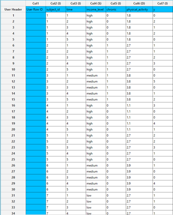
Configuration
- Select
Analytics\(\rightarrow\)Regression\(\rightarrow\)Statistical fitting\(\rightarrow\)Generalized Estimating Equations. - Set the
Type[1] of regression to Negative Binomial. - Specify the
Confidence Level (%)[2] for the test. - Specify
Max Iterations[3]. - Specify
Iterations Between Updates[4]. - Select the
Dependent Variable[5]. - Specify the
Minimum Change in Parameter Estimates[6]. - Specify the
Hessian Convergence[7]. - Specify the
Scale Parameter[8]. - Select the
Within Subject[9]. - Select the
working correlation Structureand specify the value ofMif you select M-Dependent as the correlation structure. [10]. - Select the method used to estimate the
covariance matrix[11] of the standard errors. - Select the columns by clicking on the arrow buttons [16] and moving columns between the
Excluded Columns[12] andSubjects[13] andFactors[14] andCovariates[15] lists. Specify Reference Levels[17] for the categorical factors.- Select the prefered
Formula Type[18]. Specify Custom Model Formula[19] for the analysis ifCustomoption is selected. How to specify a custom model formula?- Click on the
Executebutton [20] to perform the Negative Binomial Regression method.
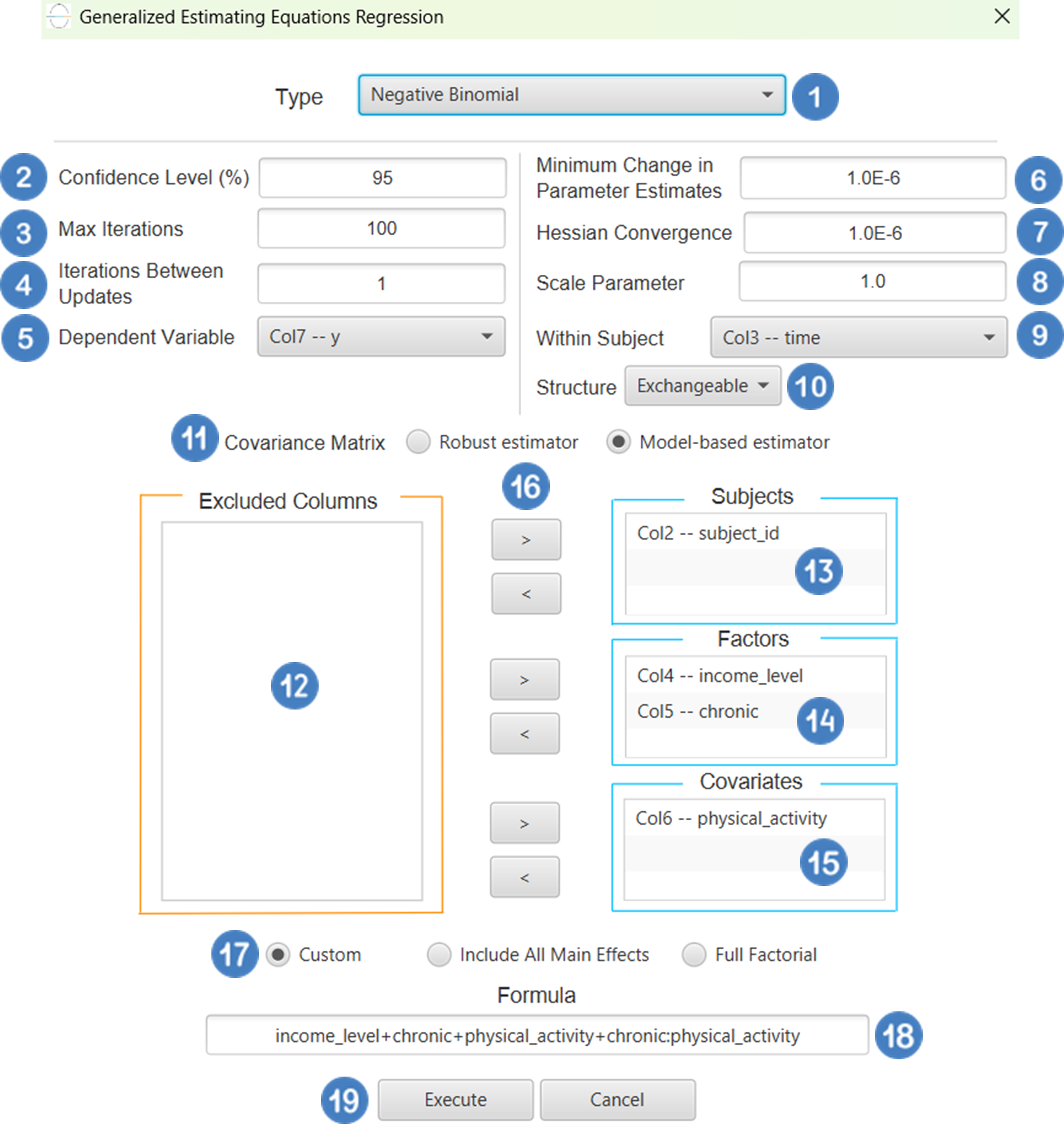
Output
The Predictions, Parameter Estimates table and Working Correlation Matrix are shown in the output spreadsheet.
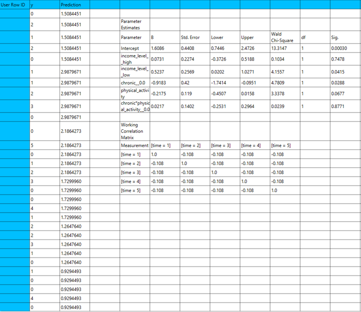
Poisson
Use the Poisson Regression method by browsing in the top ribbon:
| Analytics \(\rightarrow\) Regression \(\rightarrow\) Statistical fitting \(\rightarrow\) Generalized Estimating Equations |
And then choosing “Poisson” as the Type.
Input
All variables must be specified in the datasheet. The dependent variable must be a count variable, consisting of non-negative integer values and suitable for modeling with a Poisson distribution, as Poisson Regression within the GEE framework is used for modeling count data such as number of events, visits, or occurrences over time. Covariates should be numerical, while categorical predictors can be represented using either text labels or numeric codes. The input datasheet must include at least two columns: one for the dependent variable and one or more for the independent variables (covariates or factors). Each row should correspond to a single observation. Additionally, a subject identifier column is required to define clusters of repeated measurements, and optionally a within-subject variable to specify the order of observations within each subject. The structure of the dataset should support modeling intra-subject correlation under the Poisson distribution assumption using an appropriate link function (e.g., log link) within the GEE framework.
Configuration
| Confidence Level (%) | Specify the confidence level of the analysis. Values should range from 0 to 100 and correspond to percentages. |
| Max Iterations | Defines the maximum number of iterations the model is allowed to perform during the estimation process. If the model fails to converge before reaching this number, the algorithm stops and returns the values of the last iteration. |
| Iterations Between Updates | Defines how often the working correlation matrix is updated during estimation. |
| Dependent Variable | Select the column that corresponds to values of the dependent variable. |
| Minimum Change in Parameter Estimates | Sets the tolerance level for convergence — the smallest change in parameter estimates between iterations required to continue optimization. If the change in all parameters is below this value, the algorithm assumes convergence has been reached. |
| Hessian Convergence | Specifies a threshold for convergence based on the second derivatives (Hessian matrix). |
| Scale Parameter | Adjusts the variance of the model. |
| Within Subject | Selects the column that defines the ordering of repeated observations within each subject. |
| Structure | Defines the working correlation structure for repeated measurements within subjects. Choices include Independent, Exchangeable, AR(1), Unstructured and M-Dependent. |
| M | In the M-Dependent correlation structure, M specifies the maximum number of consecutive observations within each cluster that are assumed to be correlated, with correlations set to zero for observations more than M time points apart. M must be an integer in the range from 1 to (number of within-subject observations – 1). |
| Covariance Matrix | In the Covariance Matrix option, the user selects how the model’s standard errors will be estimated. The Robust estimator is resistant to misspecification of the correlation structure, while the Model-based estimator assumes the specified correlation is correct. |
| Subjects/Factors/Covariates/Excluded Columns | Select manually the columns that correspond to subjects, factors and the columns that correspond to covariates through the dialog window: Use the buttons to move columns between the Subjects, Factors and Covariates list and Excluded Columns list. Single-arrow buttons will move all selected columns. At least one covariate or factor column should be specified. Also, a column for the Subject is required. |
| Specify Reference Levels | Specify the reference level for each of the categorical factors specified. The default option for each factor is its last level. |
| Formula Type | These options refer to the terms that will be included in the model. The Custom option allows the user to input a formula defining the exact terms to be included. The Main Effects option allows the analysis of a model that only includes all main effects and finally, the Full Factorial option includes both all main effects and all possible interaction terms to build a full model. |
| Specify Custom Model Formula | Specify the model formula used for the analysis if the Custom option is selected. The formula is created in the Custom Formula Creation dialog window by selecting factors and covariates and adding interaction terms up to the required order. Main effects of the included columns are always part of the model and cannot be excluded. |
Output
The output of the Generalized Estimating Equations (GEEs) procedure is organized into three main sections: the Predicted Values Table, the Parameter Estimates Table and the Working Correlation Matrix.
- The Predicted Values Table shows the fitted values for the dependent variable on the specified model.
- The Parameter Estimates Table includes the estimated coefficients for the independent variables. Each row corresponds to a predictor and includes its coefficient, standard error, confidence interval, test statistic, degrees of freedom, and p-value.
- The Working Correlation Matrix displays the estimated correlations between repeated measurements of the same subject over time
Example
Input
The dataset must include a count outcome variable with non-negative integers suitable for Poisson regression. It should also include at least one independent variable (continuous or categorical), a subject identifier to group repeated measures, and a within-subject time or measurement variable to indicate observation order. The data structure should support modeling within-cluster correlation using a log link under the Poisson distribution in the GEE framework.
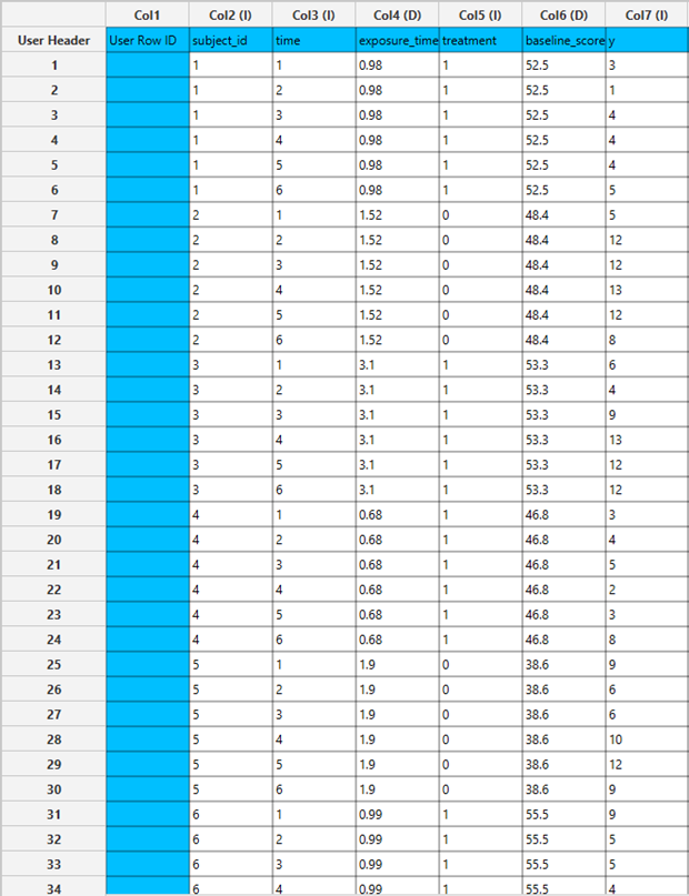
Configuration
- Select
Analytics\(\rightarrow\)Regression\(\rightarrow\)Statistical fitting\(\rightarrow\)Generalized Estimating Equations. - Set the
Type[1] of regression to Poisson. - Specify the
Confidence Level (%)[2] for the test. - Specify
Max Iterations[3]. - Specify
Iterations Between Updates[4]. - Select the
Dependent Variable[5]. - Specify the
Minimum Change in Parameter Estimates[6]. - Specify the
Hessian Convergence[7]. - Specify the
Scale Parameter[8]. - Select the
Within Subject[9]. - Select the
working correlation Structureand specify the value ofMif you select M-Dependent as the correlation structure. [10]. - Select the method used to estimate the
covariance matrix[11] of the standard errors. - Select the columns by clicking on the arrow buttons [16] and moving columns between the
Excluded Columns[12] andSubjects[13] andFactors[14] andCovariates[15] lists. Specify Reference Levels[17] for the categorical factors.- Select the prefered
Formula Type[18]. Specify Custom Model Formula[19] for the analysis ifCustomoption is selected. How to specify a custom model formula?- Click on the
Executebutton [20] to perform the Poisson Regression method.
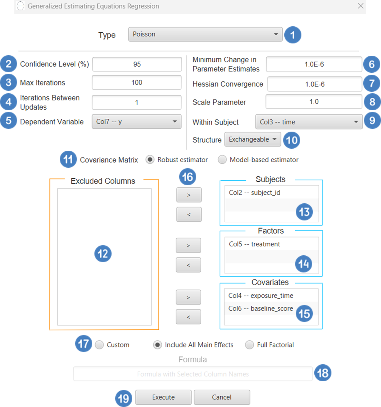
Output
The Predictions, Parameter Estimates table and Working Correlation Matrix are shown in the output spreadsheet.
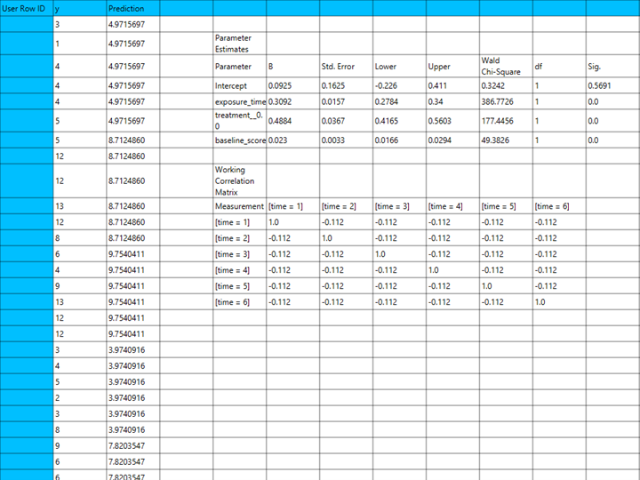
Gamma
Use the Gamma Regression method by browsing in the top ribbon:
| Analytics \(\rightarrow\) Regression \(\rightarrow\) Statistical fitting \(\rightarrow\) Generalized Estimating Equations |
And then choosing “Gamma” as the Type.
Input
All variables must be specified in the datasheet. The dependent variable must be continuous, strictly positive, and suitable for modeling with a Gamma distribution, as Gamma Regression within the GEE framework is used for positively skewed outcomes such as cost, time, or rates. Covariates should be numerical, while categorical predictors can be represented using either text labels or numeric codes. The input datasheet must include at least two columns: one for the dependent variable and one or more for the independent variables (covariates or factors). Each row should correspond to a single observation. Additionally, a subject identifier column is required to define clusters of repeated measurements, and optionally a within-subject variable to specify the order of observations within each subject. The structure of the dataset should support modeling intra-subject correlation under the Gamma distribution assumption using an appropriate link function (e.g., log link) within the GEE framework.
Configuration
| Confidence Level (%) | Specify the confidence level of the analysis. Values should range from 0 to 100 and correspond to percentages. |
| Max Iterations | Defines the maximum number of iterations the model is allowed to perform during the estimation process. If the model fails to converge before reaching this number, the algorithm stops and returns the values of the last iteration. |
| Iterations Between Updates | Defines how often the working correlation matrix is updated during estimation. |
| Dependent Variable | Select the column that corresponds to values of the dependent variable. |
| Minimum Change in Parameter Estimates | Sets the tolerance level for convergence — the smallest change in parameter estimates between iterations required to continue optimization. If the change in all parameters is below this value, the algorithm assumes convergence has been reached. |
| Hessian Convergence | Specifies a threshold for convergence based on the second derivatives (Hessian matrix). |
| Scale Parameter | Adjusts the variance of the model. |
| Within Subject | Selects the column that defines the ordering of repeated observations within each subject. |
| Structure | Defines the working correlation structure for repeated measurements within subjects. Choices include Independent, Exchangeable, AR(1), Unstructured and M-Dependent. |
| M | In the M-Dependent correlation structure, M specifies the maximum number of consecutive observations within each cluster that are assumed to be correlated, with correlations set to zero for observations more than M time points apart. M must be an integer in the range from 1 to (number of within-subject observations – 1). |
| Covariance Matrix | In the Covariance Matrix option, the user selects how the model’s standard errors will be estimated. The Robust estimator is resistant to misspecification of the correlation structure, while the Model-based estimator assumes the specified correlation is correct. |
| Subjects/Factors/Covariates/Excluded Columns | Select manually the columns that correspond to subjects, factors and the columns that correspond to covariates through the dialog window: Use the buttons to move columns between the Subjects, Factors and Covariates list and Excluded Columns list. Single-arrow buttons will move all selected columns. At least one covariate or factor column should be specified. Also, a column for the Subject is required. |
| Specify Reference Levels | Specify the reference level for each of the categorical factors specified. The default option for each factor is its last level. |
| Formula Type | These options refer to the terms that will be included in the model. The Custom option allows the user to input a formula defining the exact terms to be included. The Main Effects option allows the analysis of a model that only includes all main effects and finally, the Full Factorial option includes both all main effects and all possible interaction terms to build a full model. |
| Specify Custom Model Formula | Specify the model formula used for the analysis if the Custom option is selected. The formula is created in the Custom Formula Creation dialog window by selecting factors and covariates and adding interaction terms up to the required order. Main effects of the included columns are always part of the model and cannot be excluded. |
Output
The output of the Generalized Estimating Equations (GEEs) procedure is organized into three main sections: the Predicted Values Table, the Parameter Estimates Table and the Working Correlation Matrix.
- The Predicted Values Table shows the fitted values for the dependent variable on the specified model.
- The Parameter Estimates Table includes the estimated coefficients for the independent variables. Each row corresponds to a predictor and includes its coefficient, standard error, confidence interval, test statistic, degrees of freedom, and p-value.
- The Working Correlation Matrix displays the estimated correlations between repeated measurements of the same subject over time.
Example
Input
The dataset must include a positive continuous target variable suitable for modeling with Gamma regression. The outcome should be strictly positive and continuous, reflecting a right-skewed distribution typical of Gamma-distributed data. It should also contain at least one independent variable, which can be continuous or categorical. In addition, the dataset must include a subject identifier to group repeated observations from the same individual or unit, as well as a within-subject time or measurement indicator to reflect the longitudinal or clustered nature of the data. The structure of the dataset should allow for the modeling of within-cluster correlation using a log link function in the GEE framework.
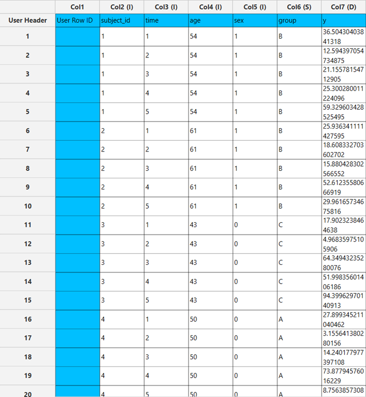
Configuration
- Select
Analytics\(\rightarrow\)Regression\(\rightarrow\)Statistical fitting\(\rightarrow\)Generalized Estimating Equations. - Set the
Type[1] of regression to Gamma. - Specify the
Confidence Level (%)[2] for the test. - Specify
Max Iterations[3]. - Specify
Iterations Between Updates[4]. - Select the
Dependent Variable[5]. - Specify the
Minimum Change in Parameter Estimates[6]. - Specify the
Hessian Convergence[7]. - Specify the
Scale Parameter[8]. - Select the
Within Subject[9]. - Select the
working correlation Structureand specify the value ofMif you select M-Dependent as the correlation structure. [10]. - Select the method used to estimate the
covariance matrix[11] of the standard errors. - Select the columns by clicking on the arrow buttons [16] and moving columns between the
Excluded Columns[12] andSubjects[13] andFactors[14] andCovariates[15] lists. Specify Reference Levels[17] for the categorical factors.- Select the prefered
Formula Type[18]. Specify Custom Model Formula[19] for the analysis ifCustomoption is selected. How to specify a custom model formula?- Click on the
Executebutton [20] to perform the Gamma Regression method.
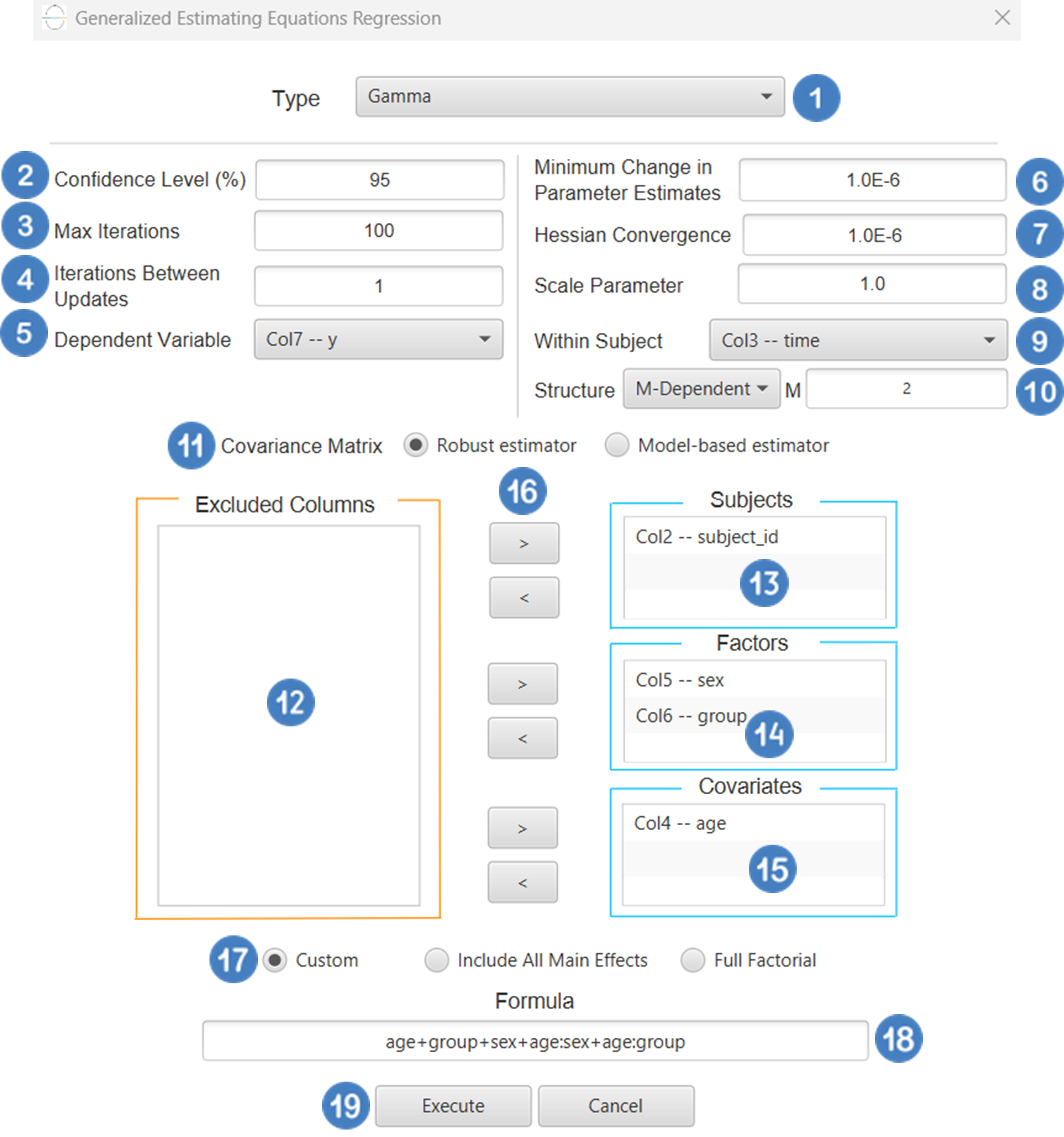
Output
The Predictions, Parameter Estimates table and Working Correlation Matrix are shown in the output spreadsheet.
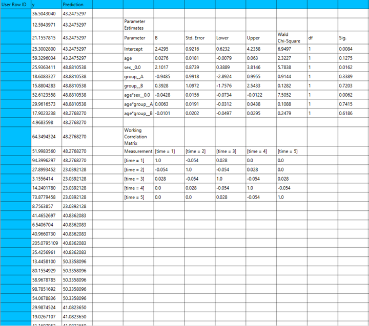
Tweedie with Identity Link
Use the Tweedie Regression method with identity link by browsing in the top ribbon:
| Analytics \(\rightarrow\) Regression \(\rightarrow\) Statistical fitting \(\rightarrow\) Generalized Estimating Equations |
And then choosing “Tweedie with Identity Link” as the Type.
Input
The dataset must be appropriately structured to support Tweedie regression with an identity link function within the framework of Generalized Estimating Equations (GEE). The dependent variable should be continuous and non-negative, and exhibit characteristics suitable for modeling with the Tweedie distribution, which is particularly well-suited to semicontinuous outcomes that contain a point mass at zero and positive continuous values. Such outcomes commonly arise in fields such as actuarial science, health economics, and environmental studies, where responses like claim amounts, medical costs, or precipitation levels often exhibit a The dataset must include at least the following components: a dependent variable, one or more independent variables (which may be numerical or categorical, with categorical variables represented as text labels or numeric codes), a subject identifier column to define clusters of repeated observations from the same unit or individual, and optionally, a within-subject measurement indicator to capture the temporal or sequential structure of the observations within each cluster. Each row in the dataset must correspond to a single observation. The data structure must support the estimation of within-cluster correlation using GEE under the Tweedie distribution with an identity link, which enables modeling of repeated or correlated data where the response variable reflects non-negative semicontinuous behavior, and where a direct, untransformed relationship between the predictors and the mean of the response is appropriate.
Configuration
| Confidence Level (%) | Specify the confidence level of the analysis. Values should range from 0 to 100 and correspond to percentages. |
| Max Iterations | Defines the maximum number of iterations the model is allowed to perform during the estimation process. If the model fails to converge before reaching this number, the algorithm stops and returns the values of the last iteration. |
| Iterations Between Updates | Defines how often the working correlation matrix is updated during estimation. |
| Dependent Variable | Select the column that corresponds to values of the dependent variable. |
| Minimum Change in Parameter Estimates | Sets the tolerance level for convergence — the smallest change in parameter estimates between iterations required to continue optimization. If the change in all parameters is below this value, the algorithm assumes convergence has been reached. |
| Hessian Convergence | Specifies a threshold for convergence based on the second derivatives (Hessian matrix). |
| Scale Parameter | Adjusts the variance of the model. |
| Within Subject | Selects the column that defines the ordering of repeated observations within each subject. |
| Structure | Defines the working correlation structure for repeated measurements within subjects. Choices include Independent, Exchangeable, AR(1), Unstructured and M-Dependent. |
| M | In the M-Dependent correlation structure, M specifies the maximum number of consecutive observations within each cluster that are assumed to be correlated, with correlations set to zero for observations more than M time points apart. M must be an integer in the range from 1 to (number of within-subject observations – 1). |
| Covariance Matrix | In the Covariance Matrix option, the user selects how the model’s standard errors will be estimated. The Robust estimator is resistant to misspecification of the correlation structure, while the Model-based estimator assumes the specified correlation is correct. |
| Subjects/Factors/Covariates/Excluded Columns | Select manually the columns that correspond to subjects, factors and the columns that correspond to covariates through the dialog window: Use the buttons to move columns between the Subjects, Factors and Covariates list and Excluded Columns list. Single-arrow buttons will move all selected columns. At least one covariate or factor column should be specified. Also, a column for the Subject is required. |
| Specify Reference Levels | Specify the reference level for each of the categorical factors specified. The default option for each factor is its last level. |
| Formula Type | These options refer to the terms that will be included in the model. The Custom option allows the user to input a formula defining the exact terms to be included. The Main Effects option allows the analysis of a model that only includes all main effects and finally, the Full Factorial option includes both all main effects and all possible interaction terms to build a full model. |
| Specify Custom Model Formula | Specify the model formula used for the analysis if the Custom option is selected. The formula is created in the Custom Formula Creation dialog window by selecting factors and covariates and adding interaction terms up to the required order. Main effects of the included columns are always part of the model and cannot be excluded. |
Output
The output of the Generalized Estimating Equations (GEEs) procedure is organized into three main sections: the Predicted Values Table, the Parameter Estimates Table and the Working Correlation Matrix.
- The Predicted Values Table shows the fitted values for the dependent variable on the specified model.
- The Parameter Estimates Table includes the estimated coefficients for the independent variables. Each row corresponds to a predictor and includes its coefficient, standard error, confidence interval, test statistic, degrees of freedom, and p-value.
- The Working Correlation Matrix displays the estimated correlations between repeated measurements of the same subject over time.
Example
Input
The dataset must include a continuous, non-negative outcome variable suitable for Tweedie regression with an identity link function. The dependent variable should reflect semicontinuous data with a mass at zero and positive continuous values, as commonly observed in applications such as insurance claims, healthcare expenditures, or environmental measures. The dataset should also include at least one independent variable, which may be continuous or categorical, a subject identifier to define clusters of repeated measurements from the same individual or unit, and a within-subject time or measurement variable to indicate the order of observations within each subject. The data structure should support the modeling of within-cluster correlation using an identity link under the Tweedie distribution in the GEE framework, allowing for a direct linear relationship between the covariates and the expected value of the outcome.
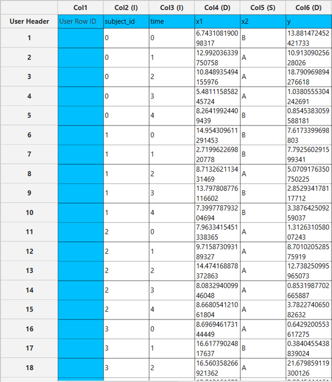
Configuration
- Select
Analytics\(\rightarrow\)Regression\(\rightarrow\)Statistical fitting\(\rightarrow\)Generalized Estimating Equations. - Set the
Type[1] of regression to Tweedie with Identity Link. - Specify the
Confidence Level (%)[2] for the test. - Specify
Max Iterations[3]. - Specify
Iterations Between Updates[4]. - Select the
Dependent Variable[5]. - Specify the
Minimum Change in Parameter Estimates[6]. - Specify the
Hessian Convergence[7]. - Specify the
Scale Parameter[8]. - Select the
Within Subject[9]. - Select the
working correlation Structureand specify the value ofMif you select M-Dependent as the correlation structure. [10]. - Select the method used to estimate the
covariance matrix[11] of the standard errors. - Select the columns by clicking on the arrow buttons [16] and moving columns between the
Excluded Columns[12] andSubjects[13] andFactors[14] andCovariates[15] lists. Specify Reference Levels[17] for the categorical factors.- Select the prefered
Formula Type[18]. Specify Custom Model Formula[19] for the analysis ifCustomoption is selected. How to specify a custom model formula?- Click on the
Executebutton [20] to perform the Tweedie Regression with Identity Link method.
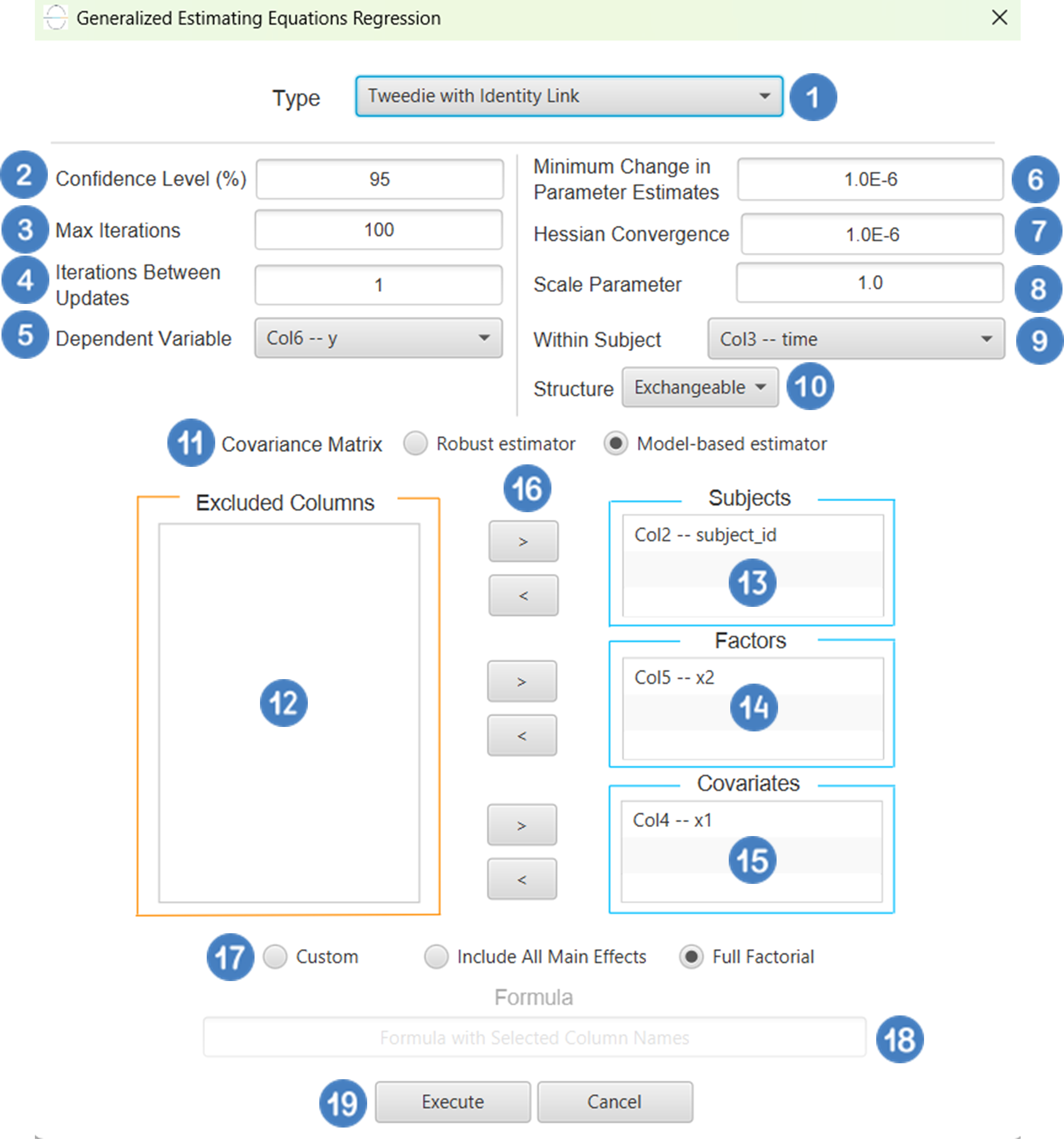
Output
The Predictions, Parameter Estimates table and Working Correlation Matrix are shown in the output spreadsheet.
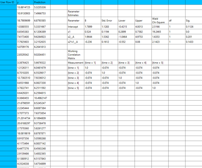
Tweedie with Log Link
Use the Tweedie Regression with Log Link method by browsing in the top ribbon:
| Analytics \(\rightarrow\) Regression \(\rightarrow\) Statistical fitting \(\rightarrow\) Generalized Estimating Equations |
And then choosing “Tweedie with Log Link” as the Type.
Input
All variables must be specified in the datasheet. The dataset must be appropriately structured to support the application of Tweedie regression with a log link function within the Generalized Estimating Equations (GEE) framework. The dependent variable should be continuous, non-negative, and exhibit characteristics consistent with the Tweedie distribution, which is particularly suitable for semicontinuous outcomes that contain a point mass at zero alongside positive continuous values. Common examples of such data include insurance claim amounts, healthcare expenditures, and rainfall measurements. The dataset must include, at minimum, the following columns: a dependent variable, one or more independent variables, which may be numeric or categorical (categorical predictors can be represented either by text labels or numeric codes), and a subject identifier that defines clusters of subject measurement indicator, representing the order or timing of observations within each cluster. Each row of the dataset should correspond to single observation. The overall structure must support the modeling of within-cluster correlation under the Tweedie distribution assumption with a log link, enabling the analysis of longitudinal or clustered data where the response variable combines features of both count and continuous distributions-such as zero inflation and positive skewness commonly observed in real world outcomes.
Configuration
| Confidence Level (%) | Specify the confidence level of the analysis. Values should range from 0 to 100 and correspond to percentages. |
| Max Iterations | Defines the maximum number of iterations the model is allowed to perform during the estimation process. If the model fails to converge before reaching this number, the algorithm stops and returns the values of the last iteration. |
| Iterations Between Updates | Defines how often the working correlation matrix is updated during estimation. |
| Dependent Variable | Select the column that corresponds to values of the dependent variable. |
| Minimum Change in Parameter Estimates | Sets the tolerance level for convergence — the smallest change in parameter estimates between iterations required to continue optimization. If the change in all parameters is below this value, the algorithm assumes convergence has been reached. |
| Hessian Convergence | Specifies a threshold for convergence based on the second derivatives (Hessian matrix). |
| Scale Parameter | Adjusts the variance of the model. |
| Within Subject | Selects the column that defines the ordering of repeated observations within each subject. |
| Structure | Defines the working correlation structure for repeated measurements within subjects. Choices include Independent, Exchangeable, AR(1), Unstructured and M-Dependent. |
| M | In the M-Dependent correlation structure, M specifies the maximum number of consecutive observations within each cluster that are assumed to be correlated, with correlations set to zero for observations more than M time points apart. M must be an integer in the range from 1 to (number of within-subject observations – 1). |
| Covariance Matrix | In the Covariance Matrix option, the user selects how the model’s standard errors will be estimated. The Robust estimator is resistant to misspecification of the correlation structure, while the Model-based estimator assumes the specified correlation is correct. |
| Subjects/Factors/Covariates/Excluded Columns | Select manually the columns that correspond to subjects, factors and the columns that correspond to covariates through the dialog window: Use the buttons to move columns between the Subjects, Factors and Covariates list and Excluded Columns list. Single-arrow buttons will move all selected columns. At least one covariate or factor column should be specified. Also, a column for the Subject is required. |
| Specify Reference Levels | Specify the reference level for each of the categorical factors specified. The default option for each factor is its last level. |
| Formula Type | These options refer to the terms that will be included in the model. The Custom option allows the user to input a formula defining the exact terms to be included. The Main Effects option allows the analysis of a model that only includes all main effects and finally, the Full Factorial option includes both all main effects and all possible interaction terms to build a full model. |
| Specify Custom Model Formula | Specify the model formula used for the analysis if the Custom option is selected. The formula is created in the Custom Formula Creation dialog window by selecting factors and covariates and adding interaction terms up to the required order. Main effects of the included columns are always part of the model and cannot be excluded. |
Output
The output of the Generalized Estimating Equations (GEEs) procedure is organized into three main sections: the Predicted Values Table, the Parameter Estimates Table and the Working Correlation Matrix.
- The Predicted Values Table shows the fitted values for the dependent variable on the specified model.
- The Parameter Estimates Table includes the estimated coefficients for the independent variables. Each row corresponds to a predictor and includes its coefficient, standard error, confidence interval, test statistic, degrees of freedom, and p-value.
- The Working Correlation Matrix displays the estimated correlations between repeated measurements of the same subject over time.
Example
Input
The dataset must include a non-negative, continuous outcome variable suitable for Tweedie regression with a log link. The dependent variable should reflect semicontinuous data with a mass at zero and positive continuous values, as seen in insurance claims, healthcare costs, or rainfall. It must also contain at least one independent variable (continuous or categorical), a subject identifier to define clusters of repeated measures, and a within-subject measurement variable to indicate the order of observations. The dataset structure should support within-cluster correlation modeling using a log link under the Tweedie distribution in the GEE framework, allowing for a multiplicative relationship between predictors and the expected outcome.
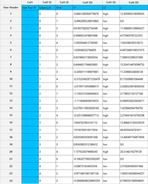
Configuration
- Select
Analytics\(\rightarrow\)Regression\(\rightarrow\)Statistical fitting\(\rightarrow\)Generalized Estimating Equations. - Set the
Type[1] of regression to Tweedie with Log Link. - Specify the
Confidence Level (%)[2] for the test. - Specify
Max Iterations[3]. - Specify
Iterations Between Updates[4]. - Select the
Dependent Variable[5]. - Specify the
Minimum Change in Parameter Estimates[6]. - Specify the
Hessian Convergence[7]. - Specify the
Scale Parameter[8]. - Select the
Within Subject[9]. - Select the
working correlation Structureand specify the value ofMif you select M-Dependent as the correlation structure. [10]. - Select the method used to estimate the
covariance matrix[11] of the standard errors. - Select the columns by clicking on the arrow buttons [16] and moving columns between the
Excluded Columns[12] andSubjects[13] andFactors[14] andCovariates[15] lists. Specify Reference Levels[17] for the categorical factors.- Select the prefered
Formula Type[18]. Specify Custom Model Formula[19] for the analysis ifCustomoption is selected. How to specify a custom model formula?- Click on the
Executebutton [20] to perform the Tweedie Regression with Log Link method.
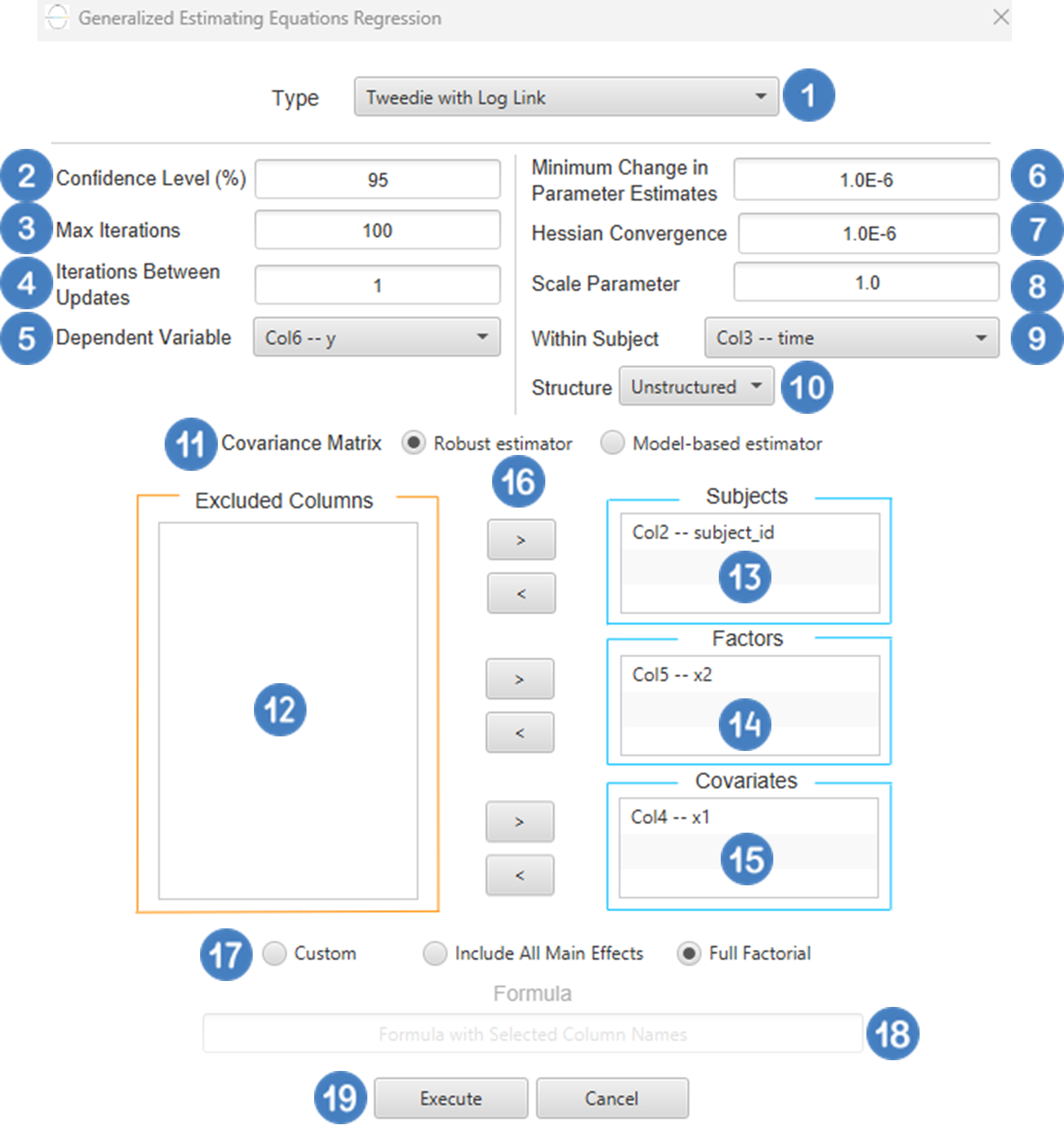
Output
The Predictions, Parameter Estimates table and Working Correlation Matrix are shown in the output spreadsheet.
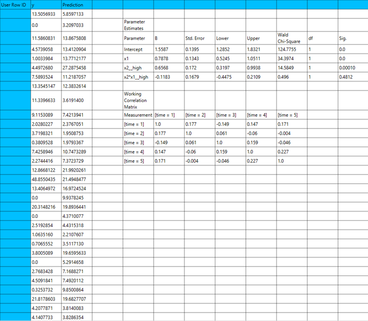
Auto ML
This function develops machine learning models for regression tasks and performs hyperparameter optimization to evaluate their performance. The models are trained and validated using all the variables of the input dataset after specification of the target variable. Additionally, the function supports multiple data splitting and normalization methods, as well as variable selection algorithms. Finally, all models are ranked according to the selected performance metrics.
Use the Auto ML function by browsing in the top ribbon:
| Analytics \(\rightarrow\) Regression \(\rightarrow\) Auto ML |
Input
Data matrix with training set data. String columns are not taken into account in the algorithm implementation, therefore categorical features must be excluded or encoded into numerical values (integer or double).
Configuration
| Available/selected models | Select manually the machine learning algorithms through the dialog window: Use the buttons to move algorithms between the Available Models and Selected Models list. Single-arrow buttons will move all selected algorithms and double-arrow buttons will move all algorithms. Available options include: k-Nearest Neighbours (kNN), Radial Basis Function Network, Linear SGD, XGBoost, Random Forest, and Fully Connected Neural Network. Double-click on each algorithm to specify the range (Min value, Max value and Step) of its hyperparameters. See more for the configuration options of each algorithm in the sections above. |
| RNG Seed | Select an integer as seed to get reproducible results. The option to select a time-based random number-generated seed is available. This seed will be used consistently for all operations within the AutoML function that require a seed. |
| Type | Select either Grid Search or the Genetic Algorithm to perform the hyperaparameter tuning. |
| Target column | Select manually from the drop-down menu the column name containing the target variable that is going to be predicted. |
| Split Method | Select manually from the drop-down menu the method for the splitting of the data into train and test sets. Available options include: Kennard-Stone, Random Partitioning, and k-Fold Partitioning. After you select the split method, specify its configuration parameters by clicking on Configure Split Method. See more for the configuration of each splitting method here. |
| Normalizer | Select manually from the drop-down menu a normalization method. Available options include: ZScore Normalizer and Min-Max Normalizer. If you select the Min-Max Normalizer, click on Configure Normalizer to specify the Min and Max values for the normalization. |
| Variable Selector | Select manually from the drop-down menu a variable selection method. Available options include: Genetic Algorithm, Boruta, Generalized Simulated Annealing, Particle Swarm Optimization, Recursive Feature Elimination, Successive Projections Algorithm, Lasso Variable Selection, MI-VIF Variable Selection, Stepwise, Best First. After you select the variable selection method, specify its configuration parameters by clicking on Configure Selector. See more for the configuration of each variable selection method here. |
| Selected Metric | Select manually from the drop-down menu the metric which will be used to evaluate the performance of each algorithm. Available options include: RSquared, MSE, RMSE, MAE, MAPE. |
| Top Results to Show | Specify how many of the algorithm ranking results, starting from the top, will be presented in the output speradsheet. |
| Number of Cores | Specify the number of CPU cores that will be used for the execution of the computations. |
Output
A ranking matrix of all the trained models including the number of top results specified in the Auto ML configuration box. The matrix presents the models starting from the top of the ranking, and consists of columns with each model’s algorithm, the variables used for the prediction of the target, and the evaluation metrics.
Example
Input
In the left-hand spreadsheet of the tab import the data matrix including the target variable for prediction. The input must include one continuous dependent variable, which will serve as the target, and at least one column with numerical values. In case that categorical-string columns are included in the set, they should be encoded into representative numerical values.
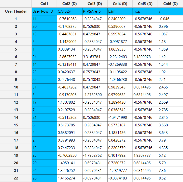
Configuration
- Select
Analytics\(\rightarrow\)Regression\(\rightarrow\)Auto ML. - Select the algorithms by clicking on the arrow buttons and moving the algorithms between the
Available ModelsandSelected Modelslists [1]. - Double-click on each algorithm to specify the range of its hyperparameters. Default values, data types (double or integer) and acceptable ranges are indicated as guidance on the input parameter values [2], [3], [4].
- Type an
RNG Seed[5] for reproducible results or a random number generatedTime-based RNG Seed. - Select the
Typeof hyperparameter optimization methods [6]. - Select the
Target Columnthat is going to be predicted from the drop-down menu [7]. - Select the
Split Methodthat will be applied on the dataset from the drop-down menu [8]. - Click on
Configure Split Methodto specify the parameters of the splitting method [9], [10]. - Select a
Normalizer[11] from the drop-down menu. If you select the Min-Max nomralizer click onConfigure Normalizerto specify the minimum and maximum values for the normalization [12], [13]. - Select a method from the
Variable Selectordrop-down menu to remove redundant prediction variables [14]. - Click on
Configure Selectorto specify the parameters for the variable selection method [15], [16]. - Select the metric which will evaluate the model performance from the
Selected Metricdrop-down menu [17]. - Type the number of
Top Results to Showfrom the model ranking [18]. - Type the
Number or Coresthat will be used to execute the computations [19]. - Click on the
Executebutton to apply the Auto ML function [20].
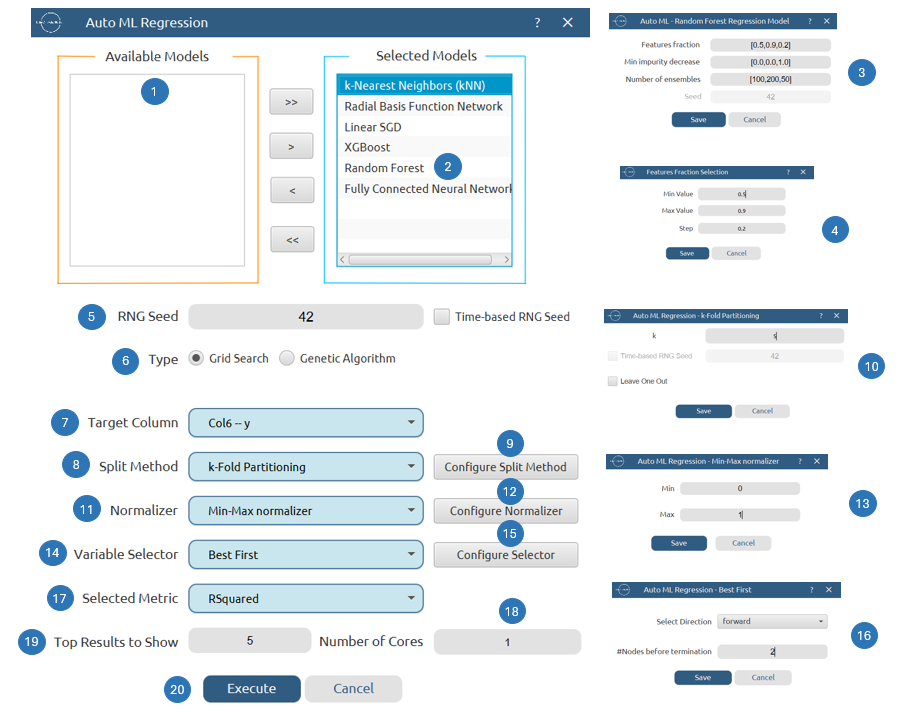
Output
In the right-hand spreadsheet of the tab the matrix with the ranking of the predictive models is presented.
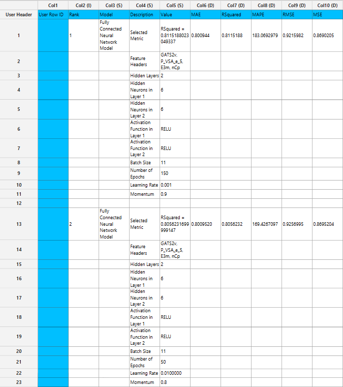
✧ Tips
- It works more efficiently for small to medium datasets and low-dimensional data. kNN is sensitive to missing data.
- The performance of the model is highly influenced by the selection of k.
- The number of neurons in the hidden layer has a high impact on the model performance, since a large number of neurons can lead to overfitting.
- It is effective in large datasets and can handle high-dimensional feature spaces. Higher learning rates may be required when Huber loss is selected, because it is less sensitive to outliers.
- Consider scaling the input data with a Z score normalizer to center them to mean and have a unit standard deviation.
- Be cautious during hyperparameter tuning: choosing smaller
etavalues, as well as increasing thelambda,alpha, andgammavalues, result in a more conservative boosting process. Increasing the value of themax depthparameter makes the model more complex and more likely to overfit.
- This algorithm performs well with datasets that contain missing values. However, it is not as efficient with a large number of sparse features or with categorical variables of many levels that are improperly encoded.
See also
The model generated by either the k Nearest Neighbors (kNN), Fully Connected Neural Network, Radial Basis Function Network, Linear SGD, XGBoost or Random Forest algorithms can be applied to any input data through the Existing Model Utilization function (e.g., a regression algorithm trained from the training set data of a machine learning model can be applied to the test/external set data).
References
- Witten Ian H and Frank, Eibe and Hall, Mark A and Pal CJ. Data Mining: Practical Machine Learning Tools and Techniques. Fourth. Morgan Kaufmann; 2011. https://doi.org/10.1016/C2009-0-19715-5.
- Murphy KP. Machine Learning: A Probabilistic Perspective. The MIT Press; 2012. 10.5555/2380985.
- Lee C-C, Chung P-C, Tsai J-R, Chang C-I. Robust radial basis function neural networks. IEEE Transactions on Systems, Man, and Cybernetics, Part B (Cybernetics) 1999;29:674–85. https://doi.org/10.1109/3477.809023.
- Ghosh J, Nag A. An Overview of Radial Basis Function Networks. In: Howlett RJ, Jain LC, editors. Radial Basis Function Networks 2: New Advances in Design, Heidelberg: Physica-Verlag HD; 2001, p. 1–36. https://doi.org/10.1007/978-3-7908-1826-0_1.
- Bottou L. Large-Scale Machine Learning with Stochastic Gradient Descent. In: Lechevallier Y, Saporta G, editors. Proceedings of COMPSTAT’2010, Heidelberg: Physica-Verlag HD; 2010, p. 177–86. https://doi.org/10.1007/978-3-7908-2604-3_16.
- XGBoost Parameters — xgboost 2.1.0-dev documentation n.d. https://xgboost.readthedocs.io/en/latest/parameter.html (accessed June 3, 2024).
- Hastie T, Tibshirani R, Friedman J. The Elements of Statistical Learning. New York, NY: Springer New York; 2009. https://doi.org/10.1007/978-0-387-84858-7.
- Chen T, Guestrin C. XGBoost: A Scalable Tree Boosting System. Proceedings of the 22nd ACM SIGKDD International Conference on Knowledge Discovery and Data Mining, 2016, p. 785–94. https://doi.org/10.1145/2939672.2939785.
- Breiman L. Random Forests. Machine Learning 2001;45:5–32. https://doi.org/10.1023/A:1010933404324.
- Nelder JA, Wedderburn RWM. Generalized linear models. J R Stat Soc A. 1972;135(3):370-84.https://doi.org/10.2307/2344614.
- McCullagh P, Nelder JA. Generalized linear models. 2nd ed. London: Chapman & Hall/CRC; 1989. https://doi.org/10.1201/9780203753736.
- McCullagh P. Regression models for ordinal data. J R Stat Soc B. 1980;42(2):109-42. https://doi.org/10.1111/j.2517-6161.1980.tb01109.x.
- Liang KY, Zeger SL. Longitudinal data analysis using generalized linear models. Biometrika. 1986;73(1):13-22. https://doi.org/10.1093/biomet/73.1.13.
Version History
Introduced in Isalos Analytics Platform v0.1.18
Instructions last updated on May 2025