Data Manipulation
This menu includes functionalities that enable the users to prepare their data for modelling and analysis. These functions correspond to standard pre-processing steps for the development of data analysis and machine learning workflows, such as data filtering, missing values filling, sorting and matrix transpose.
Remove Column(s)
This function identifies and removes columns containing redundant data. It removes included columns if there exists at least one distinct value that the percentage of its instances in the specific column is above the user-defined threshold.
Use the Remove Column(s) function by browsing in the top ribbon:
| Data Transformation \(\rightarrow\) Data Manipulation \(\rightarrow\) Remove Column(s) |
Input
Data matrix with arbitrary data requiring filtering.
Configuration
| Include/exclude columns | Select manually the columns that are going to be subject to filtering through the dialog window: Use the buttons to move columns between the Included Columns (subject to filtering) and Excluded Columns list. Single-arrow buttons will move all selected columns and double-arrow buttons will move all columns. |
| Threshold Percentage | An integer number between (0, 100) indicating the cutoff threshold. Default value: 5. |
Output
Data matrix with filtered data.
Example
Input
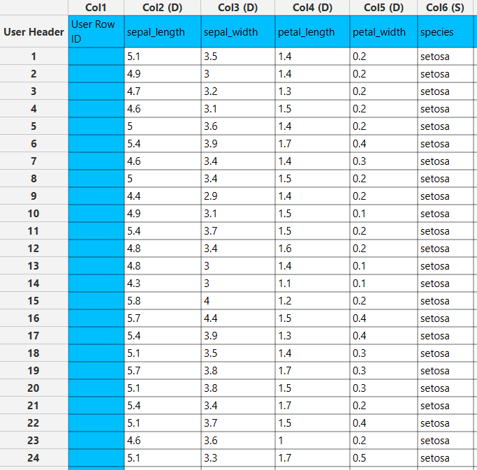
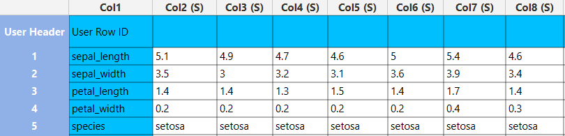
In the left-hand spreadsheet of the tab import the data matrix that is going to be filtered.
Configuration
- Select
Data Transformation\(\rightarrow\)Data Manipulation\(\rightarrow\)Remove Column(s). - Select the columns on which the filtering is going to be applied by clicking on the arrow buttons [3] and moving columns between the
Excluded Columns[1] andIncluded Columns[2] lists. In this case only columns “petal_width” and “species” are subject to filtering. - Type the threshold value in the
Threshold Percentagefield [4]. - Click on the
Executebutton [5] to apply the filtering on the selected columns.

Output
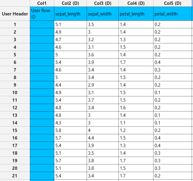
In the right-hand spreadsheet of the tab the output data matrix with the filtered columns. The Excluded Columns (“sepal_length”, “sepal_width”, and “petal_length”) remain intact in the output spreadsheet.
Select Column(s)
This function filters the input data matrix so that only the user-selected columns are passed to the output data matrix.
Use the Select Columns function by browsing in the top ribbon:
| Data Transformation \(\rightarrow\) Data Manipulation \(\rightarrow\) Select Column(s) |
Input
Data matrix with arbitrary data requiring filtering.
Configuration
| Include/exclude columns | Select manually the columns that are going to be included in the output data matrix through the dialog window: Use the buttons to move columns between the Included Columns and Excluded Columns (filtered out) list. Single-arrow buttons will move all selected columns and double-arrow buttons will move all columns. |
Output
Data matrix with filtered data.
Example
Input
In the left-hand spreadsheet of the tab import the data matrix that is going to be filtered.
Configuration
- Select
Data Transformation\(\rightarrow\)Data Manipulation\(\rightarrow\)Select Column(s). - Select the columns that are going to be filtered out by clicking on the arrow buttons [3] and moving columns between the
Excluded Columns[1] andIncluded Columns[2] lists. In this case, the columns “sepal_length”, “petal_length” and “species” are going to be included in the output spreadsheet. - Click on the
Executebutton [4] to apply the filtering on the input columns.

Output
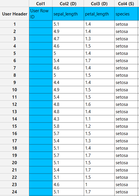
In the right-hand spreadsheet of the tab the output data matrix with the included columns “sepal_length”, “petal_length” and “species” is presented.
Matrix Transpose
This function transposes the input data table: it flips the table data by turning rows into columns and columns into rows.
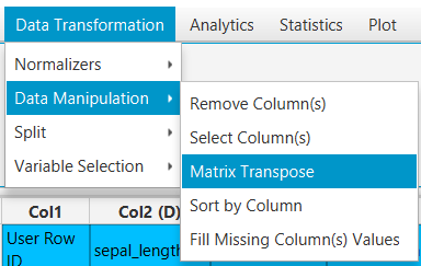
To transpose any input table, browse in the top ribbon:
| Data Transformation \(\rightarrow\) Data Manipulation \(\rightarrow\) Matrix Transpose |
Input
Data table to transpose.
Output
Table transposed by flipping rows and columns. Note that the new column types may differ from the original data types (the most general type is selected).
Example
Input
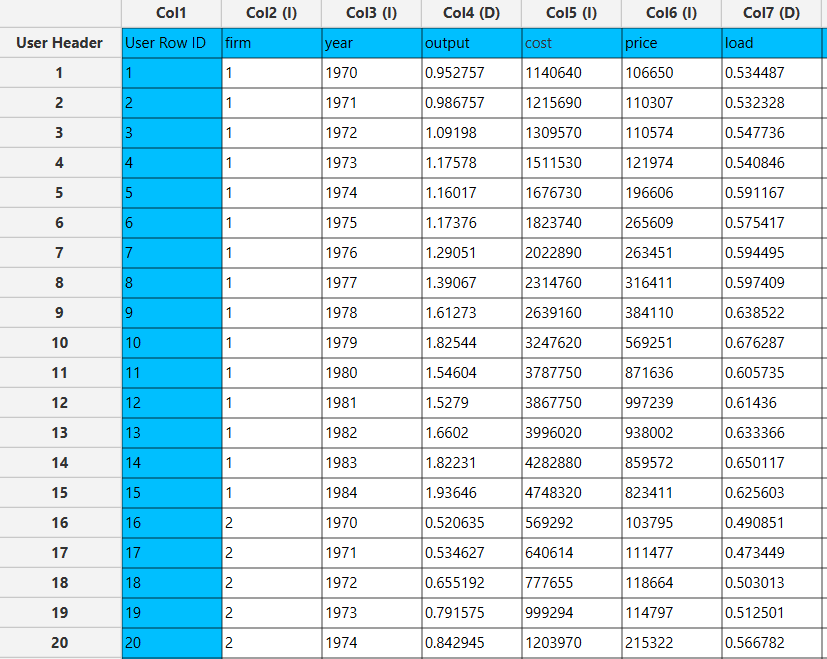
In the left-hand spreadsheet of the tab import the data table that is going to be transposed.
Configuration
- Select
Data Transformation\(\rightarrow\)Data Manipulation\(\rightarrow\)Matrix Transpose.
Output
The transposed input data table. In all columns the column type is changed to string (S).
Wide to Long Format
Wide to long format transformation is the process of restructuring a data table so that the values originally spread across multiple columns, are stacked into fewer columns and represented across multiple rows. In a wide table, repeated measurements or related variables are stored in separate columns, while in a long table these values are reorganized so that each row corresponds to one observation-variable combination. This transformation is especially useful when subsequent statistical analysis, visualization, or workflow steps require data in long format rather than in a multi-column wide structure.
Use the Wide to Long Format function by browsing in the top ribbon:
| Data Transformation \(\rightarrow\) Data Manipulation \(\rightarrow\) Wide to Long Format |
Input
Data table containing one or more identifier columns and multiple columns with values that will be stacked into long format.
Configuration
| Value Columns (Convert to Rows) | Select the wide-format columns whose values will be converted from separate columns into stacked rows in the long-format output. |
| Identifier Columns (Keep the same) | Select the column or columns that will remain unchanged in the output table and will be repeated as needed after the transformation, so that each long-format row can still be linked back to the original observation. |
| New Variable column name | Specify the name of the output column that will contain the original column headers of the transformed wide-format columns. |
| New Value column name | Specify the name of the output column that will contain the corresponding values taken from the transformed wide-format columns. |
Output
Data table in long format, where the selected wide-format columns are reshaped into a variable column and a value column, while the identifier columns are preserved. This type of structure is necessary when categorical labels and numerical values must be provided in long-form input tables.
Example
Input
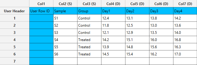
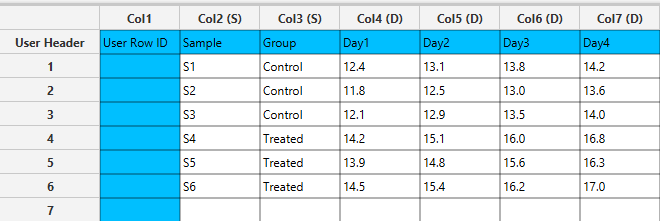
In the left-hand spreadsheet of the tab import the data table that is going to be transformed from wide to long format.
Configuration
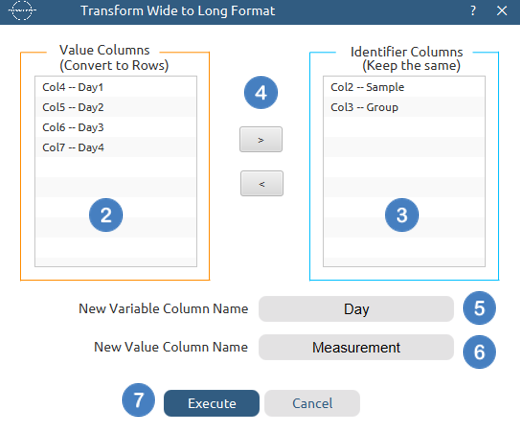
- Select
Data Transformation\(\rightarrow\)Data Manipulation\(\rightarrow\)Wide to Long Format. - Select the columns by clicking on the arrow buttons [4] and moving columns between the Value Columns [2] and Identifier Columns [3] lists.
- Specify the name [5] of the output column that will store the original column labels of the transformed variables, for example “Day”.
- Specify the name [6] of the output column that will store the corresponding values, for example “Measurement”.
- Click on the
Execute[7] button to perform the transformation.
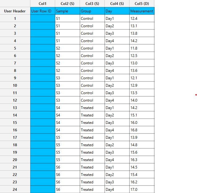
Output
The output table is converted to long format, while preserving identifier columns and stacking the selected columns into variable-value pairs.
Sort by Column
This function sorts the input data table according to a user-selected column.
To sort any input table, browse in the top ribbon:
| Data Transformation \(\rightarrow\) Data Manipulation \(\rightarrow\) Sort by Column |
Input
Data table to be sorted. Both numerical and string values are accepted.
Configuration
| Select Column | Select from the dropdown list the column name corresponding to the column according to which the data should be sorted. |
| Select Method | Select whether it should be sorted in ascending or descending order. |
Output
The sorted table.
Example
Input
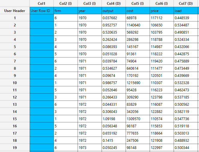
In the left-hand spreadsheet of the tab import the data table that is going to be sorted.
Configuration
- Select
Data Transformation\(\rightarrow\)Data Manipulation\(\rightarrow\)Sort by Column. - Select the query column [1] and the order method [2].
- Click on the
Executebutton [3] to sort the input table.

Output
The sorted input data table. In this case data rearrangement is performed according to the “year” column.
Fill Missing Column(s) Values
In cases of missing values in some variables, to prevent complications during statistical analysis or modeling, you can impute them using the Fill Missing Column(s) Values. The goal is to impute the missing values in a column as consistently as possible without many arbitrary decisions, so that the subsequent data analysis is not affected on the imputed values. Some standard imputation methodologies are presented bellow:
Numerical values
- Mean: Missing values are replaced by the mean value of the variable’s non-missing values within the same column.
- Mean of nearby points (or moving average): Missing values are replaced by the mean value of the cells located in the same column around the missing value cell. The range of positions (before and after the missing value cell) to be considered in the calculation is a user-defined parameter. If the nearby cells also contain missing values, then the mean value of all non-missing cells of the column is used.
- Median: Missing values are replaced by the median value of the variable’s non-missing values within the same column.
- Median of nearby points: Missing values are replaced by the median value of the cells located in the same column around the missing value cell. The range of positions (before and after the missing value cell) to be considered in the calculation is a user-defined parameter. If the nearby cells also contain missing values, then the median of all non-missing cells of the column is used.
- Linear interpolation: Missing values are filled in through linear interpolation using the values of the variables from the observation preceding and the one following the position of the missing value. This method cannot be applied if there are also rows with missing values before and/or after the row containing the missing value.
- Linear trend at point: This method is recommended for use with time series data, especially when there is a linear trend in the variable’s data in relation to the time sequence. Missing values are filled in through linear regression. In this case, the dependent variable is considered to be the variable-column itself, and the “position” of each value of the variable based on the time sequence is considered the independent variable.
Categorical values
- Most common value: This method imputes missing values with the most frequently occurring value in the dataset. It’s a straightforward approach that assumes the most common value is a reasonable estimate for the missing values.
- Existing values with same probability: In this approach, missing values are imputed randomly from the existing values in the dataset. Each existing value has an equal probability of being selected to replace the missing value.
- Existing values based on number of appearance: This method imputes missing values randomly but considering the frequency of each value in the dataset. Values are imputed based on their occurrence in the dataset, with more frequent values having a higher chance of being selected to replace missing values.
- Unique values: The missing value is replaced by a unique identifier (i.e., “Unique Value 1”, “Unique Value 2”, etc.).
To fill data gaps of any input table, browse in the top ribbon:
| Data Transformation \(\rightarrow\) Data Manipulation \(\rightarrow\) Fill Missing Column(s) Values |
Input
Data matrix with at least two columns.
Configuration
| Include/exclude columns | Select manually the columns that are going to be treated through the dialog window: Use the buttons to move columns between the Included Columns and Excluded Columns (untreated columns) list. Single-arrow buttons will move all selected columns and double-arrow buttons will move all columns. |
| Numerical Method | Select from the dropdown list the method applied on the selected columns with numerical data to fill missing values between Mean, Mean of Nearby Points, Median, Median of Nearby Points, Linear Interpolation, Linear Trend at point. |
| Span | When the Mean of Nearby Points or Median of Nearby Points is selected, type the range of cells preceding and following the missing value cell that will be used to calculate the mean and median value, respectively. |
| Categorical Method | Select from the dropdown list the method applied on the selected columns with categorical data to fill missing values between Most Common Value, Existing Values with Same Probability, Existing Values Based on Number of Appearance, Unique Values. |
Output
The data matrix with imputed missing values.
Example
Input
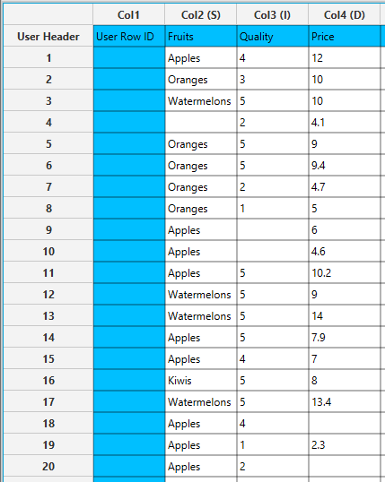
In the left-hand spreadsheet of the tab import the data table with the missing values.
Configuration
- Select
Data Transformation\(\rightarrow\)Data Manipulation\(\rightarrow\)Fill Missing Column(s) Values. - Select the columns with missing values that are going to be imputed out by clicking on the arrow buttons [3] and moving columns between the
Excluded Columns[1] andIncluded Columns[2] lists. - Select from the
Numerical Methoddropdown list [4] the method that is going to be applied to impute the missing numerical values (in this case to the missing values in the columns “Quality” and “Price”). - Select from the
Categorical Methoddropdown list [5] the method that is going to be applied to impute the missing categorical values (in this case to the missing values in the column “Fruits”). - Click on the Execute button [6] to apply the imputation methods on the input columns.

Output
In the right-hand spreadsheet of the tab, the missing values of the input table are replaced according to the configuration parameters. In this case, the missing value in “Fruits” column [1] is replaced by the label “Apples” (the most common value according to configuration) and the missing values in “Quality” and “Price” columns are replaced by 5 [2], [3] and 8.5 [4], [5], respectively (the median value of each column according to configuration).

Mathematical Calculations
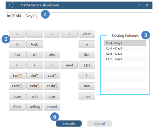
Mathematical Calculations is a data manipulation tool that allows the user to apply mathematical, trigonometric, inverse trigonometric, rounding, and statistical operations to numeric columns and constants in a dataset. It can be used either to transform values row by row or to obtain summary measures such as the mean, standard deviation, minimum, and maximum of selected data.
Use the Mathematical Calculations function by browsing in the top ribbon:
| Data Transformation \(\rightarrow\) Data Manipulation \(\rightarrow\) Mathematical Calculations |
Input
Data table containing numeric columns that will be used in the mathematical expression or calculation.
Configuration
| Existing Columns | Displays the numeric columns already present in the imported dataset, so they can be selected and inserted into the calculation expression. |
| clear | Clears the current mathematical expression from the calculator window. |
| ln | Calculates the natural logarithm of the selected value or column. |
| log | Applies a logarithmic transformation to the selected value or column. |
| √x | Calculates the square root of the selected value. |
| x | Raises the selected value to a power. |
| abs | Returns the absolute value of the selected number or expression. |
| mod | Returns the remainder after division. |
| π | Inserts the mathematical constant pi into the expression. |
| e | Inserts Euler’s number, which is the base of the natural logarithm. |
| tan(°) | Calculates the tangent of the selected value. |
| sin(°) | Calculates the sine of the selected value. |
| cos(°) | Calculates the cosine of the selected value. |
| atan | Returns the inverse tangent, meaning the angle whose tangent is the selected value. |
| asin | Returns the inverse sine, meaning the angle whose sine is the selected value. |
| acos | Returns the inverse cosine, meaning the angle whose cosine is the selected value. |
| floor | Rounds the selected value down to the nearest integer. |
| ceiling | Rounds the selected value up to the nearest integer. |
| round | Rounds the selected value to the nearest integer. |
| Σ(x) | Calculates the sum of the selected values. |
| x̄ | Calculates the arithmetic mean of the selected values. |
| Std | Calculates the standard deviation of the selected values. |
| min | Returns the minimum value from the selected data. |
| max | Returns the maximum value from the selected data. |
Output
Calculated results based on the mathematical expression defined by the user. When row-wise functions are applied to a column, the output corresponds to transformed values for each observation, while summary operators return an overall descriptive result for the selected data.
Example
Input
In the left-hand spreadsheet of the tab import the data table that is going to be used in the calculation.
Configuration
- Select
Data Transformation\(\rightarrow\)Data Manipulation\(\rightarrow\)Mathematical Calculations. - Click on the
ln[2] button to calculate the natural logarithm of the selected column. - In the
Existing Columns[3] panel select the column “Day1” to use it in the expression. - The expression is inserted into the calculator area [4] and can be edited further by adding additional operators or functions available in the panel.
- Click on the
Execute[5] button to perform the calculation.
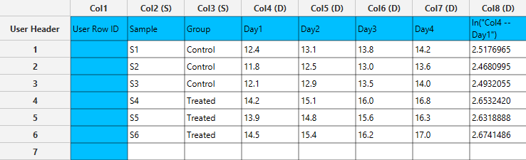
Output
The output is presented as transformed or summarized values that can be used in subsequent analysis steps.
✧ Tips
- The use of the methods
Mean of Nearby Points,Median of Nearby Points, andLinear Trend at pointis recommended when the missing values are part of a time series, but they can also be used in other cases non-restrictively.
Version History
Introduced in Isalos Analytics Platform v0.2.3
Instructions last updated on June 2024