Hypothesis Testing
Hypothesis testing is a statistical method used to decide whether the sample data sufficiently supports a particular hypothesis about a population. It generally involves formulating two competing hypotheses, the null hypothesis ($H_0$) and the alternative hypothesis ($H_a$), and then collecting data to assess the evidence. The null hypothesis ($H_0$) is the hypothesis that there is no effect or difference, and it assumes that any observed differences in the data are due to random chance. The alternative Hypothesis ($H_a$) is the hypothesis that challenges the null, proposing that there is a true effect or difference in the population.
Table of contents
- Sample Size, Mean and Standard Deviation
- One Sample T-test
- One Sample Z-test
- References
- Version History
The goal of hypothesis testing is to determine whether there is sufficient evidence to reject the null hypothesis. If the evidence is not strong enough, we fail to reject $H_0$, meaning the sample data does not provide enough proof against it.
The first step in hypothesis testing is to state the null and alternative hypotheses and then select a significance level ($a$) which represents the threshold for rejecting the null hypothesis, typically set at 0.05 (5%), meaning there’s a 5% chance of rejecting the null hypothesis when it is actually true (Type I error). Common values for $a$ are 0.05 (5%) and 0.01 (1%).
The next step involves choosing the test statistic. The test statistic depends on the nature of the data and the hypotheses being tested. Common test statistics include the Z-statistic (for large sample sizes or known population variance) and the t-statistic (for smaller sample sizes or unknown population variance).
For a Z-test:
For a t-test:
Where $\bar{x}$ is the sample mean, $\sigma$ and $s$ are the population and sample standard deviation repsectively, $n$ is the sample size and $\mu_0$ is the assumed mean of the population under the null hypothesis.
After computing the test statistic, we follow up by either calculating the p-value or comparing the test statistic with a critical value. The p-value measures the probability of obtaining a test statistic at least as extreme as the one computed, assuming the null hypothesis is true. If the p-value is less than the chosen significance level ($a$), we reject $H_0$. In some cases, you compare the test statistic directly to a critical value derived from a statistical distribution ($Z$ or $t$). If the test statistic exceeds the critical value, reject $H_0$.
There are two main types of hypothesis tests:
- One-Tailed Test. This test assesses if the population parameter is either greater than or less than a specific value. For example:
- Two-Tailed Test. This test checks for any difference, whether positive or negative, from the hypothesized value. For example:
Isalos offers three methods for conducting hypothesis tests. The first method is called Sample Size, Mean and Standard Deviation and requires the user to input the sample size, the sample mean, select whether the standard deviation is known or calculated from the sample and give its value. The software then performs a Z-test if the population standard deviation is known or a t-test if it is unknown, based on the inputted hypotheses and significance level. The second method is called One Sample T-test and involves inputting raw (sample) data. In this method, the mean and the standard deviation are automatically calculated from the sample and then a t-test for the given hypotheses and significance level is performed. Finally, the last method is called One Sample Z-test, and also involves inputting raw (sample) data. Here, only the mean is automatically calculated from the sample, while the standard deviation is given from the user, and then a Z-test for the given hypotheses and significance level is performed.
These different hypothesis testing options in Isalos offer flexibility and can accommodate a variety of testing scenarios with ease and precision. All three methods allow the user to manually specify the significance level, ensuring accurate testing for a wide range of hypotheses.
Sample Size, Mean and Standard Deviation
This method offers the flexibility to the user to input the desired sample size, mean, and standard deviation, and to choose between known ($σ$) or unknown ($s$) standard deviation. The user can also specify the significance level and the hypotheses.
Use the Sample Size, Mean and Standard Deviation for conducting Hypothesis Testing by browsing in the top ribbon:
| Statistics \(\rightarrow\) Hypothesis Testing |
And then in the Select Method option choose Sample Size, Mean and Standard Deviation.
Input
This method does not require any input in terms of raw (sample) data.
Configuration
| H$_0$: μ$_0$ | Manually insert the hypothesized mean. |
| H$_a$: μ$_a$ | Select any of the three options available for the alternative hypothesis (<, ≠, >). |
| Significance level (α) | Manually insert the significance level which may range from 0 to 1. |
| Sample size (n) | Insert the number of data points in the dataset. |
| Mean ($\bar{x}$) | Select the mean value of the dataset. |
| Standard Deviation Method | Select any of the two options available, Known StandardDeviation (σ) or Unknown StandardDeviation (s). |
| Standard Deviation | Type the value that represents the standard deviation of the data. |
Output
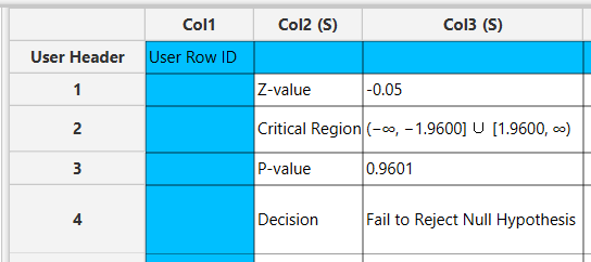
The hypothesis test is performed, and the output spreadsheet displays the test statistic, the critical region (region of rejection), the p-value, and the decision regarding the null hypothesis—whether it was rejected or not.
Example
Input
This method does not require any data to be inputted into the input spreadsheet.
Configuration
- Select
Statistics\(\rightarrow\)Hypothesis Testing. - Select
Sample Size, Mean and Standard Deviationas the desired method [1]. - Manually insert the hypothesized mean [2]
- Select from the dropdown menu one of the three available options for the alternative hypothesis $H_a$ [3]: either
<,≠or>. - Select
Significance Level (α)[4]. The value will range from 0 to 1. - Type the
Sample Size (n)[5]. - Select
Mean ($\bar{x}$)[6]. - Select one of the two available options for the
Known Standard Deviation (σ)orStandard Deviation (s)[7] : either $σ$ or $s$ will be inputted, therefore will know if standard deviation is known from population or calculated from sample. - Type the
Standard Deviation[8]. - Click on the
Executebutton [9] to perform hypothesis testing.

Output
The output data of the calculation is presented in the right-hand spreadsheet of the tab. It shows the value of the test statistic, the critical region, the p-value of the test and the decision which is whether the null hypothesis was rejected or failed to be rejected.
One Sample T-test
This method allows the user to choose the null and alternative hypotheses and the significance level to perform an one sample T-test on raw data, that are stored in a single column.
Use the One Sample T-test method for performing hypothesis testing by browsing in the top ribbon:
| Statistics \(\rightarrow\) Hypothesis Testing |
And then in the Select Method option choose One Sample T-test.
Input
This method only allows hypothesis testing for a single column therefore users should fill the desired column with numerical values and not nominal values.
Configuration
| H$_0$: μ$_0$ | Manually insert the hypothesized mean. |
| H$_a$: μ$_a$ | Select any of the three options available for the alternative hypothesis (<, ≠, >). |
| Significance level (α) | Manually insert the significance level which may range from 0 to 1. |
| Target Column | Select which column you want to perform hypothesis testing on. |
Output
The hypothesis test is performed, and the output spreadsheet displays the test statistic, the critical region (region of rejection), the p-value, and the decision regarding the null hypothesis—whether it was rejected or not.
Example
Input
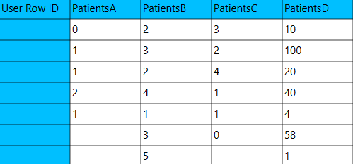
The left-hand spreadsheet contains a column that is populated with the necessary to perform the One Sample T-test on.
Configuration
- Select
Statistics\(\rightarrow\)Hypothesis Testing. - Select
One Sample T-testas the desired method [1]. - Manually insert the hypothesized mean [2].
- Select one of the three available options for the alternative hypothesis $H_a$ [3]: either
<,≠or>. - Select
Significance Level (α)[4]. The value will range from 0 to 1. - Select the
Target column[5] to perform hypothesis testing on. - Click on the
Executebutton [6] to perform hypothesis testing.

Output
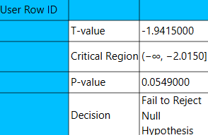
The output data of the calculation is presented in the right-hand spreadsheet of the tab. It shows the value of the test statistic, the critical region, the p-value of the test and the decision which is whether the null hypothesis was rejected or failed to be rejected.
One Sample Z-test
This method allows the user to specify the null and alternative hypotheses, the significance level of the test and the population’s standard deviation (σ) to perform an one sample Z-test on raw data, that are stored in a single column.
Use the One Sample Z-test method for performing hypothesis testing by browsing in the top ribbon:
| Statistics \(\rightarrow\) Hypothesis Testing |
And then in the Select Method option choosing One Sample Z-test.
Input
This method only allows hypothesis testing for a single column therefore users should fill the desired column with numerical values and not nominal values.
Configuration
| H$_0$: μ$_0$ | Manually insert the hypothesized mean. |
| H$_a$: μ$_a$ | Select any of the three options available for the alternative hypothesis (<, ≠, >). |
| Significance level (α) | Manually insert the significance level which may range from 0 to 1. |
| Target Column | Select which column you want to perform hypothesis testing on. |
| Population Standard Deviation (σ) | Type the the standard deviation of the population which is a non-negative real number. |
Output
The hypothesis test is performed, and the output spreadsheet displays the test statistic, the critical region (region of rejection), the p-value, and the decision regarding the null hypothesis—whether it was rejected or not.
Example
Input
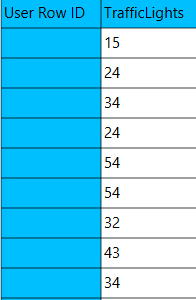
The left-hand spreadsheet contains a column that is populated with the necessary to perform the One Sample Z-test on.
Configuration
- Select
Statistics\(\rightarrow\)Hypothesis Testing. - Select
One Sample Z-testas the desired method [1]. - Manually insert the hypothesized mean [2].
- Select one of the three available options for the alternative hypothesis $H_a$ [3]: either
<,≠or>. - Select
Significance Confidence Level (α)[4]. The value will range from 0 to 1. - Select the
Target Column[5] to perform hypothesis testing on. - Manually insert the
Population Standard Deviation (σ)[6]. - Click on the
Executebutton [7] to perform hypothesis testing.

Output
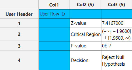
The output data of the calculation is presented in the right-hand spreadsheet of the tab. It shows the value of the test statistic, the critical region, the p-value of the test and the decision which is whether the null hypothesis was rejected or failed to be rejected.
References
- Moore, DS, McCabe, GP. Introduction to the practice of statistics. WH Freeman/Times Books/Henry Holt & Co.; 1989.
- Bluman, A. Elementary Statistics: A step by step approach 9e. McGraw Hill.; 2014.
Version History
Introduced in Isalos Analytics Platform v0.4.0
Instructions last updated on December 2024