Probability Distribution Functions
Isalos provides tools to explore probability distribution functions across a wide range of well-known distribution families, including options to customize parameters for each distribution. This flexibility allows users to model specific scenarios, analyse different shapes of distributions, and observe how changes in parameters affect the distribution’s behaviour. Isalos also provides the ability to plot the probability mass function (PDF) or probability density function (PDF) and the cumulative distribution function (CDF) of a random variable of a known distribution for the parameters that the user has inputted.
A probability distribution is a mathematical description of the probabilities of events, which are subsets of the sample space—the set of all possible outcomes of a random phenomenon. To define probability distributions, two primary functions are used: the probability mass function (PMF) or probability density function (PDF), and the cumulative distribution function (CDF). The choice between the PMF and PDF depends on whether the random variable has a discrete or continuous sample space.
The probability distribution of a discrete random variable is characterized by a probability mass function which is a function that returns the probability of the random variable taking each value separately. For example, for a random variable $X$ the PMF is given as below:
For a continuous random variable, the probability distribution is defined by the probability density function (PDF). While the PDF does not give the probability that $X$ takes a specific value (since for a continuous variable $𝑃(𝑋=𝑥) = 0$), it provides a measure of relative likelihood. For a continuous random variable $𝑋$, the PDF is defined as:
The cumulative distribution function (CDF) of a random variable, whether continuous or discrete, gives the probability that the variable takes a value less than or equal to a specified value. For both types of random variables, having either the PMF/PDF or the CDF is sufficient to describe the distribution, as they can be derived from one another as follows:
For a discrete random variable:
For a continuous random variable:
Another useful function in probability and statistics is the inverse cumulative distribution function (ICDF), also known as the quantile function. The ICDF is the inverse of the cumulative distribution function (CDF) and returns the value of the random variable $𝑋$ at which the cumulative probability is equal to a specified probability $𝑝$. Formally, for a given probability $𝑝$ (where $0 \leq 𝑝 \leq 1$), the ICDF is defined as:
Distributions with particular properties or those frequently encountered in practical applications are often given specific names and are characterized by certain parameters. For example, the Normal distribution is defined by its mean ($μ$) and standard deviation ($σ$), which determine the distribution’s center and spread, respectively. Similarly, the Binomial distribution models the number of successes in a fixed number of independent trials, with parameters $𝑛$ (number of trials) and $𝑝$ (probability of success on each trial).
These named distributions are often accompanied by closed-form expressions for their PMFs or PDFs, making them useful in both theoretical and applied statistics. They allow for easier calculations of probabilities and expectations and provide important approximations for complex distributions. Additionally, many of these distributions have well-known cumulative distribution functions (CDFs) and can be transformed or manipulated using their parameters to fit specific data types or research needs.
Binomial Distribution
The Binomial distribution is a statistical distribution that describes the number of successes ($k$) in a sequence of $n$ independent experiments, which are also called Bernoulli trials, each with a Boolean-valued outcome: success (with probability $p$) or failure (with probability $1-p$). Since the values of $k$ are non-negative integers, therefore the binomial distribution is a discrete probability distribution and has the following PMF:
Where $k$ is the number of successes, $k∈{0,1,2,3,…,n}$, $n$ is the number of trials, $n∈{1,2,3,…}$ and $p$ is the probability of success for each trial, $p∈[0,1]$.
Calculate the distribution functions for the binomial distribution by browsing through the ribbon:
| Statistics \(\rightarrow\) Probability Distribution Function |
And then choosing Binomial Distribution.
Input
If the Single Value option is chosen then this method does not require any input in terms of raw (sample) data. Otherwise, input the multiple values for each parameter in a separate column in the input spreadsheet according to what are the accepted values for each parameter.
Configuration
| Single Value/Multiple Values | Choose whether to manually input the parameters of the distribution or take multiple values for them through the input sheet. |
| Plot Chart | Select any of the five available options (No Chart/Line Chart Horizontal, Line Chart Vertical, Bar Chart Horizontal, Bar Chart Vertical) to create a chart for the PMF and CDF for the specified parameters. |
| Number of successes | Insert the Number of successes. Acceptable values are only integers from 0 to the Number of trials ($n$). Can only be used if the No chart option is selected in the Plot Chart section. |
| Number of trials | Insert the Number of trials. Acceptable values are only positive integers. |
| Success probability per trial | Insert the Success probability per trial. Acceptable values are real numbers from 0 to 1. |
| ICDF Calculation | You can tick/select the box if you also want to calculate the ICDF for a specific probability. |
| Probability of X successes | If the ICDF calculation is selected, you will be asked to specify the probability for which you want to calculate the ICDF on. Acceptable values are real numbers from 0 to 1. |
Output
If the No chart option is selected then the output of the method will be the PMF and CDF of the binomial distribution for parameters $n$ (number of trials) and $p$ (success probability per trial) as given, calculated on the specified number of successes ($k$). In the output spreadsheet there is also the mean and the variance for the distribution and if the ICDF option is selected then the outcome of the function for the specified probability is also presented. If any other Plot Chart option is selected, then the method returns the plots for the PMF and CDF and in the output spreadsheet returns the PMF and CDF calculated on all possible values for the number of successes while also providing the mean and the variance of the distribution and the outcome of the ICDF if selected.
Example
Input
This method does not require any data to be inputted into the input spreadsheet if the Single Value option is chosen.
Configuration
- Select
Statistics\(\rightarrow\)Probability Distribution Functions. - Select
Binomial Distributionas the desired distribution [1] from the dropdown menu. - Select/tick
Single Value/Multiple Valuesto select whether to input the values for the distribution manually or insert multiple values for each parameter from the input sheet. [2]. - Select one of the five available options for
Plot Chart[3] (No Chart/Line Chart Horizontal,Line Chart Vertical,Bar Chart Horizontal,Bar Chart Vertical) to specify if a chart for the PMF and CDF is required and the type of it. - Select
Number of Successes[4] if theNo chartoption is selected. The value should be an integer from 0 the number of trials ($n$). - Select
Number of trials[5]. The value should be a positive integer. - Select
Success probability per trial[6]. The value should range from 0 to 1. - Select/tick if to perform an
ICDF calculation[7] for a specific probability. - If the ICDF calculation is selected, specify the probability of X successes [8] you want to calculate the ICDF on. The value should range from 0 to 1.
- Click on the
Executebutton [9] to calculate the results.

Output
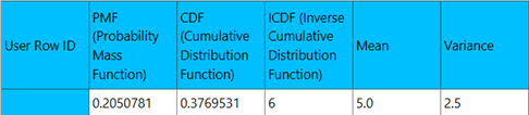
The output data of the calculation is presented in the right-hand spreadsheet of the tab. It shows the value of PMF and the CDF for the specified number of successes $k$, the value of the ICDF for the specified probability and the mean and variance of the binomial distribution with parameters $n$ (number of trials) and $p$ (success probability per trial) as specified.
Erlang Distribution Special Case of Gamma Distribution
The Erlang Distribution is a special case of the Gamma distribution in which the shape of the distribution is discretized. It is a two-parameter family of continuous probability distributions with support $x∈[0,∞)$. There are two ways in which this distribution is described either by the “shape” $k$ which is a positive integer and the “rate” $λ$ which is a positive real number or instead of using $λ$, the reciprocal of the rate is sometimes used instead and is called “scale” $β$. The Erlang distribution is the distribution of $k$ independent exponential variables with mean $1/λ$ each. Therefore, if the shape parameter $k$ is 1 the Erlang distribution is the same as the Exponential distribution. The PDF for both parametrizations of the distribution is given as below:
Where $k$ is the “shape” of the distribution, $k∈{1,2,3,…}$, $λ$ is the “rate” of the distribution $λ∈(0,∞)$ and $x$ is the support $x∈[0,∞)$.
Or
Where $k$ is the “shape” of the distribution, $k ∈{1,2,3,…}$, $β$ is the “scale” of the distribution $β∈(0,∞)$ and $x$ is the support $x∈[0,∞)$.
Calculate the distribution functions for the Erlang distribution by browsing through the ribbon:
| Statistics \(\rightarrow\) Probability Distribution Function |
And then choosing Erlang Distribution Special Case of Gamma Distribution.
Input
If the Single Value option is chosen then this method does not require any input in terms of raw (sample) data. Otherwise, input the multiple values for each parameter in a separate column in the input spreadsheet according to what are the accepted values for each parameter.
Configuration
| Single Value/Multiple Values | Choose whether to manually input the parameters of the distribution or take multiple values for them through the input sheet. |
| Parameter type | Select any of the two available options rate/scale to specify which parametrization of the distribution to use. |
| Plot Chart | Select any of the five available options (No Chart/Line Chart Horizontal, Line Chart Vertical, Bar Chart Horizontal, Bar Chart Vertical) to create a chart for the PMF and CDF for the specified parameters. |
| Support | Insert the Support. Acceptable values range in $[0,∞)$. |
| Shape | Insert the Shape of the distribution. Acceptable values are positive integers. |
| Rate/Scale | Insert the Rate/Scale of the distribution according to which Parameter type was chosen. Acceptable values range in $(0,∞)$. |
| ICDF Calculation | You can tick/select the box if you also want to calculate the ICDF for a specific probability. |
| Cumulative probability | If the ICDF calculation is selected, you will be asked to specify the probability for which you want to calculate the ICDF on. Acceptable values are real numbers from 0 to 1. |
Output
If the No chart option is selected then the output of the method will be the PDF and CDF of the Erlang distribution for parameters $k$ (shape) and $λ/β$ (rate/scale according to which option was chosen) as given, calculated on the specified support ($x$). In the output spreadsheet there is also the mean and the variance for the distribution and if the ICDF option is selected then the outcome of the function for the specified probability is also presented. If any other Plot Chart option is selected, then the method returns the plots for the PDF and CDF and in the output spreadsheet returns the PDF and CDF calculated on a wide range of acceptable values of support while also providing the mean and the variance of the distribution and the outcome of the ICDF if selected.
Example
Input
If the Single Value option is chosen then this method does not require any data to be inputted into the input spreadsheet.
Configuration
- Select
Statistics\(\rightarrow\)Probability Distribution Functions. - Select
Erlang Distribution Special Case of Gamma Distributionas the desired distribution [1] from the dropdown menu. - Select/tick
Single Value/Multiple Valuesto select whether to input the values for the distribution manually or insert multiple values for each parameter from the input sheet [2]. - Select the
Parameter type[3] to choose which parametrization of the distribution to be used. - Select one of the five available options for
Plot Chart[4] (No Chart/Line Chart Horizontal,Line Chart Vertical,Bar Chart Horizontal,Bar Chart Vertical) to specify if a chart for the PDF and CDF is required and the type of it. - Select
Support[5] if theNo chartoption is selected. The value should range in $[0,∞)$. - Select
Shape[6]. The value should be a positive integer. - Select
Rate/Scale[7] according to whichParameter Typewas chosen. The value should range in $(0,∞)$. - Select/tick if to perform an
ICDF calculation[8] for a specific probability. - If the
ICDF calculationis selected, specify theCumulative probability[9] which is the probability you want to calculate the ICDF on. The value should range from 0 to 1. - Click on the
Executebutton [10] to calculate the results.

Output
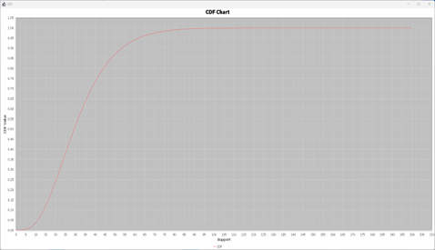
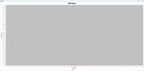
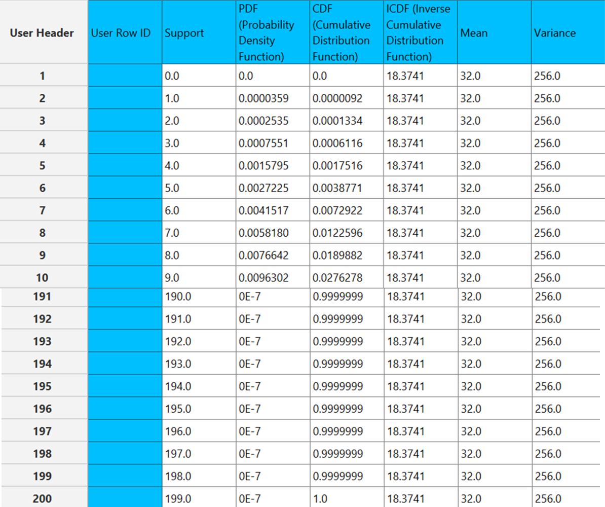
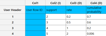
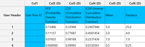
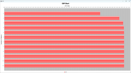
The two graphs produced are presented in two separate windows and the calculations generated are shown in the right-hand spreadsheet of the tab. This includes the PDF and CDF calculated for 200 different values of support (we present only the first and last 10), the calculation of the ICDF for the given probability and the mean and variance of the distribution.
Exponential Distribution
The exponential distribution models the probability distribution of intervals between events in a Poisson point process, where events happen independently and continuously at a fixed average rate. It can also be seen as a special case of the Gamma distribution and is the continuous counterpart of the geometric distribution. Notably, the exponential distribution has a memoryless property—the probability of an event occurring in a future interval does not depend on how much time has already passed, meaning past events have no effect on future probabilities. The PDF for the Exponential Distribution is given as below:
Where $λ$ is the rate or inverse scale of the distribution, $λ∈(0,∞)$ and $x$ is the support $x∈[0,∞)$.
Calculate the distribution functions for the Exponential distribution by browsing through the ribbon:
| Statistics \(\rightarrow\) Probability Distribution Function |
And then choosing Exponential Distribution.
Input
If the Single Value option is chosen then this method does not require any input in terms of raw (sample) data. Otherwise, input the values for each parameter in a separate column in the input spreadsheet according to what are the accepted values for each parameter.
Configuration
| Single Value/Multiple Values | Choose whether to manually input the parameters of the distribution or take multiple values for them through the input sheet. |
| Plot Chart | Select any of the five available options (No Chart/Line Chart Horizontal, Line Chart Vertical, Bar Chart Horizontal, Bar Chart Vertical) to create a chart for the PMF and CDF for the specified parameters. |
| Support | Insert the Support. Acceptable values range in $[0,∞)$. |
| Rate/Inverse scale | Insert the Rate/Inverse scale of the distribution. Acceptable values range in $(0,∞)$. |
| Success probability per trial | Insert the Success probability per trial. Acceptable values are real numbers from 0 to 1. |
| ICDF Calculation | You can tick/select the box if you also want to calculate the ICDF for a specific probability. |
| Cumulative probability | If the ICDF calculation is selected, you will be asked to specify the probability for which you want to calculate the ICDF on. Acceptable values are real numbers from 0 to 1. |
| icdf at probability | If the ICDF calculation is selected, you will be asked to specify the probability for which you want to calculate the ICDF on. Acceptable values are real numbers from 0 to 1. |
Output
If the No chart option is selected then the output of the method will be the PDF and CDF of the Exponential distribution for parameter $λ$ (rate/inverse scale) as given, calculated on the specified support ($x$). In the output spreadsheet there is also the mean and the variance for the distribution and if the ICDF option is selected then the outcome of the function for the specified probability is also presented. If any other Plot Chart option is selected, then the method returns the plots for the PDF and CDF and in the output spreadsheet returns the PDF and CDF calculated on a wide range of acceptable values of support while also providing the mean and the variance of the distribution and the outcome of the ICDF if selected.
Example
Input
Input the values for each parameter in a separate column in the input spreadsheet according to what are the accepted values for each parameter.
Configuration
- Select
Statistics\(\rightarrow\)Probability Distribution Functions. - Select
Exponential Distributionas the desired distribution [1] from the dropdown menu. - Select/tick
Single Value/Multiple Valuesto select whether to input the values for the distribution manually or insert multiple values for each parameter from the input sheet. [2]. - Select the column that corresponds to values for
Support[3]. The values should be range in $[0,∞)$. - Select the column that corresponds to values
Rate/Inverse scale[4]. The values should be range in $(0,∞)$. - Select/tick if to perform an
ICDF calculation[5] for a specific probability. - If the
ICDF calculationis selected, select the column that corresponds to values for the cumulative probability [6] which is the probability you want to calculate the ICDF on. The values should range from 0 to 1. - Click on the
Executebutton [7] to calculate the results.

Output
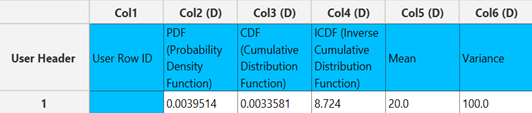
The output data of the calculation is presented in the right-hand spreadsheet of the tab. It shows the value of PDF and the CDF for each value of support $x$ and rate $λ$, the value of the ICDF for each value of the cumulative probability and the mean and variance of the exponential distribution with parameter $λ$, for each value of $λ$.
Gamma Distribution
The Gamma Distribution is a two-parameter family of continuous probability distributions with support $x∈[0,∞)$. There are two ways in which this distribution is described either by the “shape” $k/α$ which is a positive integer and the “scale” $θ$ which is a positive real number or instead of using $θ$, an inverse scale parameter is used $β = 1/θ$, called “rate”. The exponential distribution, Erlang distribution, and chi-squared distribution are special cases of the gamma distribution. The PDF for both parametrizations of the distribution is given as below:
Where $k$ is the “shape” of the distribution, $k∈(0,∞)$, $θ$ is the “scale” of the distribution $θ∈(0,∞)$ and x is the support $x∈[0,∞)$.
Or
Where $α$ is the “shape” of the distribution, $α∈(0,∞)$, $β$ is the “rate” of the distribution $β∈(0,∞)$ and $x$ is the support $x∈[0,∞)$.
Calculate the distribution functions for the Gamma distribution by browsing through the ribbon:
| Statistics \(\rightarrow\) Probability Distribution Function |
And then choosing Gamma Distribution.
Input
If the Single Value option is chosen then this method does not require any input in terms of raw (sample) data. Otherwise, input the values for each parameter in a separate column in the input spreadsheet according to what are the accepted values for each parameter.
Configuration
| Single Value/Multiple Values | Choose whether to manually input the parameters of the distribution or take multiple values for them through the input sheet. |
| Parameter type | Select any of the two available options k and theta/alpha and beta to specify which parametrization of the distribution to use. |
| Plot Chart | Select any of the five available options (No Chart/Line Chart Horizontal, Line Chart Vertical, Bar Chart Horizontal, Bar Chart Vertical) to create a chart for the PDF and CDF for the specified parameters. |
| Support | Insert the Support. Acceptable values range in $[0,∞)$. |
| Shape | Insert the Shape of the distribution. Acceptable values range in $(0,∞)$. |
| Scale/Rate | Insert the Scale/Rate of the distribution according to which Parameter Type was chosen. Acceptable values range in $(0,∞)$. |
| ICDF Calculation | You can tick/select the box if you also want to calculate the ICDF for a specific probability. |
| Cumulative probability | If the ICDF calculation is selected, you will be asked to specify the probability for which you want to calculate the ICDF on. Acceptable values are real numbers from 0 to 1. |
Output
If the No chart option is selected then the output of the method will be the PDF and CDF of the Gamma distribution for parameters $k/α$ (shape) and $θ/β$ (scale/rate according to which option was chosen) as given, calculated on the specified support ($x$). In the output spreadsheet there is also the mean and the variance for the distribution and if the ICDF option is selected then the outcome of the function for the specified probability is also presented. If any other Plot Chart option is selected, then the method returns the plots for the PDF and CDF and in the output spreadsheet returns the PDF and CDF calculated on a wide range of acceptable values of support while also providing the mean and the variance of the distribution and the outcome of the ICDF if selected.
Example
Input
If the Single Value option is chosen then this method does not require any data to be inputted into the input spreadsheet.
Configuration
- Select
Statistics\(\rightarrow\)Probability Distribution Functions. - Select
Gamma Distributionas the desired distribution [1] from the dropdown menu. - Select/tick
Single Value/Multiple Valuesto select whether to input the values for the distribution manually or insert multiple values for each parameter from the input sheet [2]. - Select the
Parameter type[3] to choose which parametrization of the distribution to be used. - Select one of the five available options for
Plot Chart[4] (No Chart/Line Chart Horizontal,Line Chart Vertical,Bar Chart Horizontal,Bar Chart Vertical) to specify if a chart for the PDF and CDF is required and the type of it. - Select
Support[5] if theNo chartoption is selected. The value should range in $[0,∞)$. - Select
Shape[6]. The value should range in $(0,∞)$. - Select
Scale/Rate[7] according to the chosenParameter type. The value should range in $(0,∞)$. - Select/tick if to perform an
ICDF calculation[8] for a specific probability. - If the
ICDF calculationis selected, specify theCumulative probability[9] which is the probability you want to calculate the ICDF on. The value should range from 0 to 1. - Click on the
Executebutton [10] to calculate the results.

Output
The output data of the calculation is presented in the right-hand spreadsheet of the tab. It shows the value of PDF and the CDF for the specified support $x$, the value of the ICDF for the specified probability and the mean and variance of the gamma distribution with parameters $k$ (shape) and $θ$ (scale) as specified.
Geometric Distribution
The Geometric distribution refers to one of two discrete probability distributions, each modeling different aspects of Bernoulli trials—experiments with two outcomes, success or failure, repeated independently.
The probability distribution of the number $X$ of Bernoulli trials needed to get one success, supported on $N = {1,2,3,…}$ with the following PMF:
Where $k$ is the number of trials, $k∈{1,2,3,…}$, and $p$ is the probability of success for each trial, $p∈[0,1]$.
The probability distribution of the number $Y = X – 1$ of failures before the first success, supported on $N_0=0,1,2,3,…$ with the following PMF:
Where $k$ is the number of failures, $k∈{0,1,2,3,…}$, and $p$ is the probability of success for each trial, $p∈[0,1]$.
These two distributions differ in interpretation: the first counts the total trials needed for the first success (often called the shifted geometric distribution), while the second counts only the failures prior to the first success. It’s essential to distinguish between them, as they reflect slightly different perspectives on the number of trials and failures leading to the first success in a series of Bernoulli trials.
Calculate the distribution functions for the Geometric distribution by browsing through the ribbon:
| Statistics \(\rightarrow\) Probability Distribution Function |
And then choosing Geometric Distribution.
Input
If the Single Value option is chosen then this method does not require any input in terms of raw (sample) data. Otherwise, input the values for each parameter in a separate column in the input spreadsheet according to what are the accepted values for each parameter.
Configuration
| Single Value/Multiple Values | Choose whether to manually input the parameters of the distribution or take multiple values for them through the input sheet. |
| Parameter type | Select any of the two available options Number of trials/Number of failures to choose which version of geometric distribution to use. |
| Plot Chart | Select any of the five available options (No Chart/Line Chart Horizontal, Line Chart Vertical, Bar Chart Horizontal, Bar Chart Vertical) to create a chart for the PMF and CDF for the specified parameters. |
| Number of trials/failures | Insert the Number of trials/Number of failures according to which parameter type was chosen. Acceptable values are only positive integers for number of trials and non-negative integers for number of failures. Can only be used if the No chart option is selected in the Plot Chart section. |
| Success probability | Insert the Success probability. Acceptable values are real numbers from 0 to 1. |
| ICDF Calculation | You can tick/select the box if you also want to calculate the ICDF for a specific probability. |
| Probability of X trials/failures | If the ICDF calculation is selected, you will be asked to specify the probability for which you want to calculate the ICDF on. Acceptable values are real numbers from 0 to 1. |
Output
If the No chart option is selected then the output of the method will be the PMF and CDF of the Geometric distribution for parameters $k$ (number of trials/failures) and $p$ (success probability per trial) as given. In the output spreadsheet there is also the mean and the variance for the distribution and if the ICDF option is selected then the outcome of the function for the specified probability is also presented. If any other Plot Chart option is selected, then the method returns the plots for the PMF and CDF and in the output spreadsheet returns the PMF and CDF calculated on all possible values for the number of trials/failures until first success while also providing the mean and the variance of the distribution and the outcome of the ICDF if selected.
Example
Input
If the Single Value option is chosen then this method does not require any data to be inputted into the input spreadsheet.
Configuration
- Select
Statistics\(\rightarrow\)Probability Distribution Functions. - Select
Geometric Distributionas the desired distribution [1] from the dropdown menu. - Select/tick
Single Value/Multiple Valuesto select whether to input the values for the distribution manually or insert multiple values for each parameter from the input spreadsheet [2]. - Select any of the two available options
Number of trials/Number of failuresforParameter type[3] to choose which version of geometric distribution to use. - Select one of the five available options for
Plot Chart[4] (No Chart/Line Chart Horizontal,Line Chart Vertical,Bar Chart Horizontal,Bar Chart Vertical) to specify if a chart for the PMF and CDF is required and the type of it. - Select
Number of trials/Number of failures[5] if the No chart option is selected according to which Parameter type was chosen. The value should be an integer larger or equal to 1 for the number of trials and an integer larger or equal to 0 for the number of failures. - Select
Success probability[6]. The value should range from 0 to 1. - Select/tick if to perform an
ICDF calculation[7] for a specific probability. - If the
ICDF calculationis selected, specify the probability of $X$ trials/failures [8] you want to calculate the ICDF on. The value should range from 0 to 1. - Click on the
Executebutton [9] to calculate the results.

Output
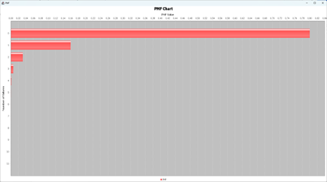
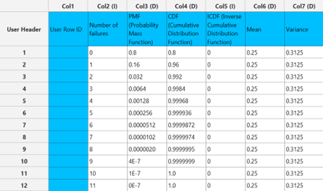
The two graphs produced are presented in two separate windows and the calculations generated are shown in the right-hand spreadsheet of the tab. This includes the PMF and CDF calculated for 12 different values of the number of failures, the calculation of the ICDF for the given probability and the mean and variance of the distribution.
Negative Binomial Distribution
The Negative binomial distribution is a discrete probability distribution that models the number of failures in a sequence of Bernoulli trials before a specified number of successes ($r$). The PMF of the Negative Binomial distribution is defined as follows:
Where $k$ is the number of failures, $k∈{0,1,2,3,…,n}$, $r$ is the number of successes, $n∈{1,2,3,…}$ and $p$ is the probability of success for each trial, $p∈[0,1]$.
Calculate the distribution functions for the Negative Binomial distribution by browsing through the ribbon:
| Statistics \(\rightarrow\) Probability Distribution Function |
And then choosing Negative Binomial Distribution.
Input
If the Single Value option is chosen then this method does not require any input in terms of raw (sample) data. Otherwise, input the values for each parameter in a separate column in the input spreadsheet according to what are the accepted values for each parameter.
Configuration
| Single Value/Multiple Values | Choose whether to manually input the parameters of the distribution or take multiple values for them through the input sheet. |
| Plot Chart | Select any of the five available options (No Chart/Line Chart Horizontal, Line Chart Vertical, Bar Chart Horizontal, Bar Chart Vertical) to create a chart for the PMF and CDF for the specified parameters. |
| Number of successes | Insert the Number of successes. Acceptable values are only positive integers. |
| Number of failures | Insert the Number of failures. Acceptable values are only non-negative integers. Can only be used if the No chart option is selected in the Plot Chart section. |
| Success probability per trial | Insert the Success probability per trial. Acceptable values are real numbers from 0 to 1. |
| ICDF Calculation | You can tick/select the box if you also want to calculate the ICDF for a specific probability. |
| Probability of X failures | If the ICDF calculation is selected, you will be asked to specify the probability for which you want to calculate the ICDF on. Acceptable values are real numbers from 0 to 1. |
Output
If the No chart option is selected then the output of the method will be the PMF and CDF of the negative binomial distribution for parameters $r$ (number of successes) and $p$ (success probability per trial) as given, calculated on the specified number of failures ($k$). In the output spreadsheet there is also the mean and the variance for the distribution and if the ICDF option is selected then the outcome of the function for the specified probability is also presented. If any other Plot Chart option is selected, then the method returns the plots for the PMF and CDF and in the output spreadsheet returns the PMF and CDF calculated on all possible values for the number of failures while also providing the mean and the variance of the distribution and the outcome of the ICDF if selected.
Example
Input
If the Single Value option is chosen then this method does not require any data to be inputted into the input spreadsheet.
Configuration
- Select
Statistics\(\rightarrow\)Probability Distribution Functions. - Select
Negative Binomial Distributionas the desired distribution [1] from the dropdown menu. - Select/tick
Single Value/Multiple Valuesto select whether to input the values for the distribution manually or insert multiple values for each parameter from the input sheet. [2] - Select one of the five available options for
Plot Chart(No Chart/Line Chart Horizontal,Line Chart Vertical,Bar Chart Horizontal,Bar Chart Vertical) to specify if a chart for the PMF and CDF is required and the type of it. - Select
Number of Successes[4]. The value should be a positive integer. - Select
Number of failures[5] if the No chart option is selected. The value should be a non-negative integer. - Select
Success probability per trial[6]. The value should range from 0 to 1. - Select/tick if to perform an
ICDF calculation[7] for a specific probability. - If the
ICDF calculationis selected, specify theProbability of X failures[8] you want to calculate the ICDF on. The value should range from 0 to 1. - Click on the
Executebutton [9] to calculate the results.

Output
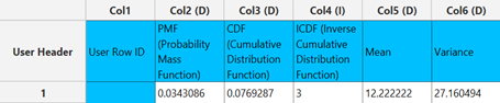
The output data of the calculation is presented in the right-hand spreadsheet of the tab. It shows the value of PMF and the CDF for the specified number of failures $k$, the value of the ICDF for the specified probability and the mean and variance of the negative binomial distribution with parameters $r$ (number of successes) and $p$ (success probability per trial) as specified.
Normal Distribution
The Normal distribution, also known as the Gaussian distribution, describes a symmetrical plot of data around its mean value, where the width of the curve is defined by the standard deviation. It is a two-parameter family of continuous distributions with the parameters being $μ$, the mean or expectation of the distribution and $\sigma$, the standard deviation of the distribution. The PDF of the normal distribution is defined as follows:
Where $μ$ is the mean of the distribution, $μ∈(-∞,∞)$ and $σ$ is the standard deviation of the distribution, $σ∈(0,∞)$.
Calculate the distribution functions for the Normal distribution by browsing through the ribbon:
| Statistics \(\rightarrow\) Probability Distribution Function |
And then choosing Normal Distribution.
Input
If the Single Value option is chosen then this method does not require any input in terms of raw (sample) data. Otherwise, input the values for each parameter in a separate column in the input spreadsheet according to what are the accepted values for each parameter.
Configuration
| Single Value/Multiple Values | Choose whether to manually input the parameters of the distribution or take multiple values for them through the input sheet. |
| Plot Chart | Select any of the five available options (No Chart/Line Chart Horizontal, Line Chart Vertical, Bar Chart Horizontal, Bar Chart Vertical) to create a chart for the PMF and CDF for the specified parameters. |
| Support | Insert the Support. Acceptable values any real numbers. Can only be used if the No chart option is selected in the Plot Chart section. |
| Mean | Insert the Mean of the distribution. Acceptable values are any real numbers. |
| Standard deviation | Insert the Standard deviation of the distribution. Acceptable values are positive real numbers. |
| ICDF Calculation | You can tick/select the box if you also want to calculate the ICDF for a specific probability. |
| Cumulative probability | If the ICDF calculation is selected, you will be asked to specify the probability for which you want to calculate the ICDF on. Acceptable values are real numbers from 0 to 1. |
Output
If the No chart option is selected then the output of the method will be the PDF and CDF of the Normal distribution for parameters $μ$ (mean) and $σ$ (standard deviation) as given, calculated on the specified support ($x$). In the output spreadsheet there is also the mean and the variance for the distribution and if the ICDF option is selected then the outcome of the function for the specified probability is also presented. If any other Plot Chart option is selected, then the method returns the plots for the PDF and CDF and in the output spreadsheet returns the PDF and CDF calculated wide range of values of support while also providing the mean and the variance of the distribution and the outcome of the ICDF if selected.
Example
Input
If the Single Value option is chosen then this method does not require any data to be inputted into the input spreadsheet.
Configuration
- Select
Statistics\(\rightarrow\)Probability Distribution Functions. - Select
Normal Distributionas the desired distribution [1] from the dropdown menu. - Select/tick
Single Value/Multiple Valuesto select whether to input the values for the distribution manually or insert multiple values for each parameter from the input sheet [2]. - Select one of the five available options for
Plot Chart[3] (No Chart/Line Chart Horizontal,Line Chart Vertical,Bar Chart Horizontal,Bar Chart Vertical) to specify if a chart for the PDF and CDF is required and the type of it. - Select
Support[4] if theNo chartoption is selected. The value should be a real number. - Select
Mean[5]. The value should be a real number. - Select
Standard Deviation[6]. The value should a positive real number. - Select/tick if to perform an
ICDF calculation[7] for a specific probability. - If the
ICDF calculationis selected, specify the Cumulative probability [8] you want to calculate the ICDF on. The value should range from 0 to 1. - Click on the
Executebutton [9] calculate the results.

Output
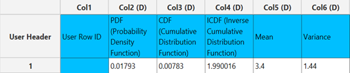
The output data of the calculation is presented in the right-hand spreadsheet of the tab. It shows the value of PDF and the CDF for the specified support $x$, the value of the ICDF for the specified probability and the mean and variance of the normal distribution with parameters $μ$ (mean) and $σ$ (standard deviation) as specified.
Poisson Distribution
The Poisson Distribution is a discrete probability distribution that describes the probability of a given number of events occurring in a fixed interval of time if these events occur with a known constant mean rate and independently of the time since the last event. The PMF of the Poisson Distribution is given as below:
Where $k$ is the number of occurrences, $k∈{0,1,2,3,…,n}$ and $λ$ is the mean rate of occurrence, $λ∈ [0,∞)$.
Calculate the distribution functions for the Poisson Distribution by browsing through the ribbon:
| Statistics \(\rightarrow\) Probability Distribution Function |
And then choosing Poisson Distribution.
Input
If the Single Value option is chosen then this method does not require any input in terms of raw (sample) data. Otherwise, input the values for each parameter in a separate column in the input spreadsheet according to what are the accepted values for each parameter.
Configuration
| Single Value/Multiple Values | Choose whether to manually input the parameters of the distribution or take multiple values for them through the input sheet. |
| Plot Chart | Select any of the five available options (No Chart/Line Chart Horizontal, Line Chart Vertical, Bar Chart Horizontal, Bar Chart Vertical) to create a chart for the PMF and CDF for the specified parameters. |
| Number of occurrences | Insert the Number of occurrences. Acceptable values are only non-negative integers. Can only be used if the No chart option is selected in the Plot Chart section. |
| Rate | Insert the Rate of the distribution. Acceptable values are only non-negative real numbers. |
| ICDF Calculation | You can tick/select the box if you also want to calculate the ICDF for a specific probability. |
| Probability of X occurrences | If the ICDF calculation is selected, you will be asked to specify the probability for which you want to calculate the ICDF on. Acceptable values are real numbers from 0 to 1. |
Output
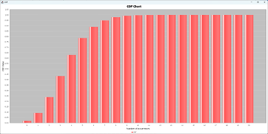
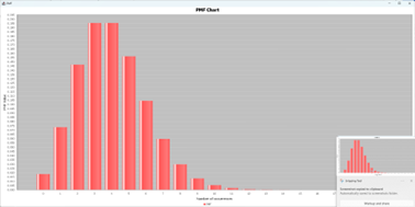
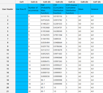
If the No chart option is selected then the output of the method will be the PMF and CDF of the Poisson Distribution for parameter $λ$ (mean rate of occurrence), calculated on the specified number of occurrences ($k$). In the output spreadsheet there is also the mean and the variance for the distribution and if the ICDF option is selected then the outcome of the function for the specified probability is also presented. If any other Plot Chart option is selected, then the method returns the plots for the PMF and CDF and in the output spreadsheet returns the PMF and CDF calculated on all possible values for the number of occurrences while also providing the mean and the variance of the distribution and the outcome of the ICDF if selected.
Example
Input
If the Single Value option is chosen then this method does not require any data to be inputted into the input spreadsheet.
Configuration
- Select
Statistics\(\rightarrow\)Probability Distribution Functions. - Select
Poisson Distributionas the desired distribution [1] from the dropdown menu. - Select/tick
Single Value/Multiple Valuesto select whether to input the values for the distribution manually or insert multiple values for each parameter from the input sheet [2]. - Select one of the five available options for
Plot Chart[3] (No Chart/Line Chart Horizontal,Line Chart Vertical,Bar Chart Horizontal,Bar Chart Vertical) to specify if a chart for the PMF and CDF is required and the type of it. - Select
Number of occurrences[4] if theNo chartoption is selected. The value should be a non-negative integer. - Select
Rate[5]. The value should be a non-negative real number. - Select/tick if to perform an
ICDF calculation[6] for a specific probability. - If the
ICDF calculationis selected, specify theProbability of X occurrences[7] you want to calculate the ICDF on. The value should range from 0 to 1. - Click on the
Executebutton [8] to calculate the results.

Output
The two graphs produced are presented in two separate windows and the calculations generated are shown in the right-hand spreadsheet of the tab. This includes the PMF and CDF calculated for 21 different values of support, the calculation of the ICDF for the given probability and the mean and variance of the distribution.
Uniform Distribution
The uniform distribution is a family of symmetric probability distributions which describe an experiment where there is an arbitrary outcome that lies between certain bounds. The bounds are defined by the parameters of the distribution, a and b, which are the lower and upper limits. The PDF of the Uniform Distribution is defined as follows:
Where $x$ is the support, $x∈(-∞,∞)$, a is the lower limit of the distribution, $a∈(-∞,∞)$, and $b$ is the upper limit of the distribution, $b∈(-∞,∞)$ with the constraint that $a<b$.
Calculate the distribution functions for the Uniform distribution by browsing through the ribbon:
| Statistics \(\rightarrow\) Probability Distribution Function |
And then choosing Uniform Distribution.
Input
If the Single Value option is chosen then this method does not require any input in terms of raw (sample) data. Otherwise, input the values for each parameter in a separate column in the input spreadsheet according to what are the accepted values for each parameter.
Configuration
| Single Value/Multiple Values | Choose whether to manually input the parameters of the distribution or take multiple values for them through the input sheet. |
| Plot Chart | Select any of the five available options (No Chart/Line Chart Horizontal, Line Chart Vertical, Bar Chart Horizontal, Bar Chart Vertical) to create a chart for the PDF and CDF for the specified parameters. |
| Support | Insert the Support. Acceptable values are any real numbers. Can only be used if the No chart option is selected in the Plot Chart section. |
| Lower limit | Insert the Lower limit of the distribution. Acceptable values any real numbers. |
| Upper limit | Insert the Upper limit of the distribution. Acceptable values any real numbers. |
| ICDF Calculation | You can tick/select the box if you also want to calculate the ICDF for a specific probability. |
| Cumulative probability | If the ICDF calculation is selected, you will be asked to specify the probability for which you want to calculate the ICDF on. Acceptable values are real numbers from 0 to 1. |
Output
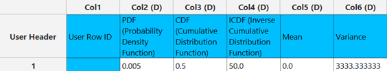
If the No chart option is selected then the output of the method will be the PDF and CDF of the uniform distribution for parameters $a$ (lower limit) and $b$ (upper limit) as given, calculated on the specified support ($x$). In the output spreadsheet there is also the mean and the variance for the distribution and if the ICDF option is selected then the outcome of the function for the specified probability is also presented. If any other Plot Chart option is selected, then the method returns the plots for the PDF and CDF and in the output spreadsheet returns the DMF and CDF calculated wide range of values of support while also providing the mean and the variance of the distribution and the outcome of the ICDF if selected.
Example
Input
If the Single Value option is chosen then this method does not require any data to be inputted into the input spreadsheet.
Configuration
- Select
Statistics\(\rightarrow\)Probability Distribution Functions. - Select
Uniform Distributionas the desired distribution [1] from the dropdown menu. - Select/tick
Single Value/Multiple Valuesto select whether to input the values for the distribution manually or insert multiple values for each parameter from the input sheet [2]. - Select one of the five available options for
Plot Chart[3] (No Chart/Line Chart Horizontal,Line Chart Vertical,Bar Chart Horizontal,Bar Chart Vertical) to specify if a chart for the PDF and CDF is required and the type of it. - Select
Support[4] if theNo chartoption is selected. The value should be a real number. - Select
Lower limit[5]. The value should be a real number. - Select
Upper Limit[6]. The value should be a real number with the constraint that (Lower limit<Upper limit). - Select/tick if to perform an
ICDF calculation[7] for a specific probability. - If the ICDF calculation is selected, specify the
Cumulative probability[8] you want to calculate the ICDF on. The value should range from 0 to 1. - Click on the
Executebutton [9] to calculate the results.

Output
The output data of the calculation is presented in the right-hand spreadsheet of the tab. It shows the value of PDF and the CDF for the specified support $x$, the value of the ICDF for the specified probability and the mean and variance of the uniform distribution with parameters $a$ (Lower limit) and $b$ (Upper limit) as specified.
References
- Moore, D. S., McCabe, G. P., & Craig, B. A. Introduction to the Practice of Statistics (10th ed.). New York: W. H. Freeman; 2021.
- Bluman, A. G. Elementary Statistics: A Step by Step Approach (10th ed.). New York: McGraw-Hill Education; 2018.
Version History
Introduced in Isalos Analytics Platform v0.4.0
Instructions last updated on January 2025