Space Filling
Space-Filling Designs are a type of Design of Experiments (DoE) used to explore a wide range of factor combinations in a systematic and efficient way. The goal is to ensure that the experimental points are distributed evenly across the entire factor space, maximizing the coverage of possible factor levels. These designs are particularly useful when the underlying model is unknown or when the focus is on understanding the behavior of a system across a broad spectrum of conditions.
Halton Design
Halton designs utilize Halton sequences, which are low-discrepancy sequences that generate quasi-random points in a multidimensional space. These sequences are deterministic, but they have the advantage of distributing points more uniformly compared to traditional random sampling methods. The low-discrepancy nature ensures that the design points cover the experimental space more evenly, which is particularly valuable when exploring high-dimensional systems where evenly distributed data points improve the quality of experimental results.
In the context of DοΕ, Halton sequences are used to address challenges such as efficiently sampling large parameter spaces and improving the convergence of optimization algorithms. The quasi-random nature of the sequence allows experimenters to explore the design space in a structured manner, avoiding clustering or gaps that can occur with random sampling.
Halton sequences are generated by applying a radical-inverse function in different prime-number bases. Each dimension of the design space is assigned a different prime base, which ensures that the points in the space are distributed without overlap or repetition.
For instance, in base-2, the following steps are followed to compute the $n^{th}$ sample for a factor that takes values within the range $[a,b]$:
- Convert the integer $n$ to its base-2 representation.
- Reverse the digits of the base-2 number.
- Interpret the reversed digits as a fraction.
- Scale the fraction using the formula $𝑎 + ( 𝑏 – 𝑎 ) × fraction$, which maps the value to the desired range.
This process is repeated for each dimension, ensuring that the points are spread across the entire design space.
One of the significant advantages of Halton sequences in DοE is their ability to provide uniform coverage of the experimental space with relatively fewer points compared to traditional designs. This makes them especially useful in applications where the design space is large and computational or experimental costs are high or there is a need to minimize the number of experiments while maintaining a good representation of the entire space.
Although Halton designs are not directly tied to Response Surface Methodology (RSM), they can be employed as part of the experimental designs used to collect data for response surface modelling. Halton sequences are particularly useful when initial exploration of the design space is required, or when a broad set of points is needed to fit a global model. By efficiently exploring the space, Halton designs can help identify important regions of interest, which can then be refined using more traditional RSM approaches, such as Central Composite Designs (CCD) or Box-Behnken Designs.
Use the Halton Design by browsing in the top ribbon:
| DOE \(\rightarrow\) Space Filling \(\rightarrow\) Halton Design |
Input
Numerical values should be specified in the input datasheet. Halton design is applied when at least one factor (column) is specified along with at least two levels/values (rows).
Configuration
| Number of Center Points per Block | Select manually the Number of Center Points per Block to be included in the output list of experiments. There is no minimum requirement or any other limitation. |
| Number of Replicates | Select manually the Number of Replicates which represents the number of times to replicate the entire design. This value should be an integer, and the lowest acceptable value is 1. |
| Number of Blocks | Select from the list of available options the Number of Blocks. These designs can only be blocked on replicates, so the available options include 1 and the selected Number of Replicates. |
| Number of Samples | Select manually the Number of Samples to be included in the output list of experiments. The lowest value that can get is 1. |
| Random Standard order | You can tick/select the box if randomness is required in the output list of experiments. |
| Time-based RNG Seed | If randomness is selected, then you have the option to also tick/select the box to set the random generated number seed based on time. |
| RNG Seed | Select manually the random generated number seed if required. |
| Include/exclude columns | Select manually the columns through the dialog window: Use the buttons to move columns between the Included Columns and Excluded Columns list. Single-arrow buttons will move all selected columns and double-arrow buttons will move all columns. |
Output
A list of experiments (combinations) is generated in the output datasheet along with the Block number, the Replicate Number, the Standard order and the Point type of each experiment based on the Halton design.
Example
Input
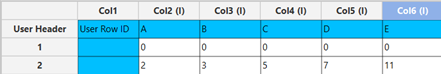
In the input datasheet minimum requirement is to specify one factor (column) and insert minimum two levels (values) for each factor (column), as shown below.
Configuration
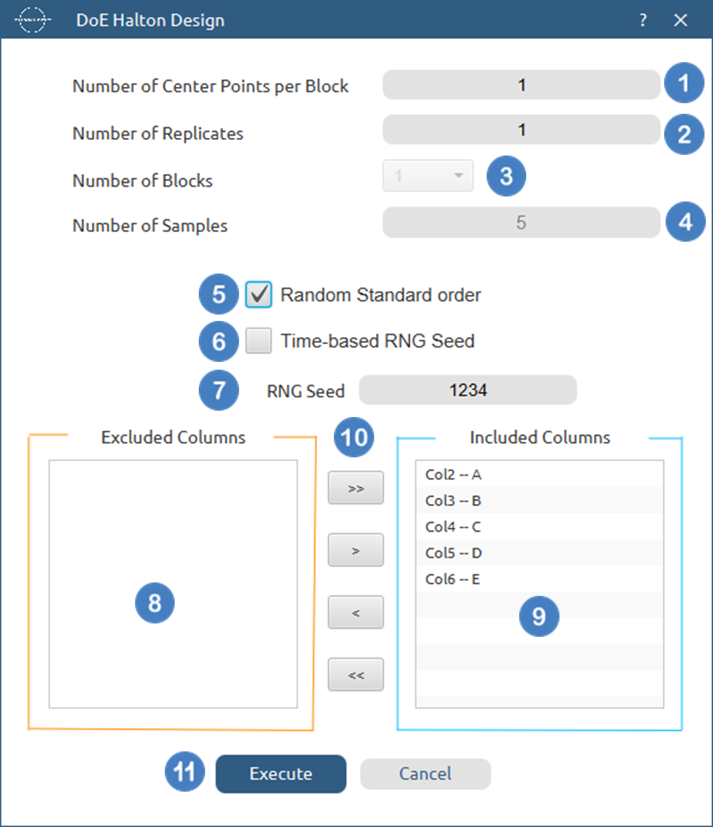
- Select
DOE\(\rightarrow\)Space Filling\(\rightarrow\)Halton Design. - Select the
Number of Center Points per Block[1] to be generated in the output list of experiments. - Select the
Number of Replicates[2]. The lowest value that can be set is 1. - Select the
Number of Blocks[3]. - Select the
Number of Samples[4] to be included in the output list of experiments. The lowest value that can get is 1. - Select/tick if required the
Random Standard order[5] to imply randomness in the output list of experiments. - If randomness is selected either select/tick to generate the number seed for randomness based on time [6] or by manually setting a value [7].
- Select the columns by clicking on the arrow buttons [10] and moving columns between the
Excluded Columns[8] andIncluded Columns[9] lists. - Click on the
Executebutton [11] to perform Halton design method.
Output
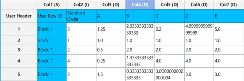
A list of experiments (combinations) is generated in the output datasheet along with the Block number based on the Halton design method selected. Standard Order, Block number, Replicate Number and Point Type are presented in Cols 2,3,4 and 5 accordingly as shown below.
LHS
Latin Hypercube Sampling (LHS) is a stratified sampling technique that ensures uniform coverage of each factor’s range in a multidimensional space. LHS divides the range of each input variable into n equally spaced intervals, where n is the number of observations or sample points. One of the key features of LHS is that for each input variable, exactly one sample is drawn from each interval. This ensures that the entire range of each factor is well covered without any clustering of points, which can often occur in purely random sampling methods.
A Latin Hypercube of $n$ runs for $k$ factors is represented by an $n × k$ matrix, each column of which is a permutation of n equally spaced levels. Typically , the n levels are taken to be:
Given an $n × k$ Latin Hypercube $L = (l_{ij})$, a Latin hypercube design $D$ in the design space $[a_1, b_1] \times \cdots \times [a_k, b_k]$ ($[a_j, b_j]$ is the range of the $j^{th}$ factor) can be generated and the design matrix of $D$ is an $n × k$ matrix with the $(i, j)^{th}$ entry being:
where $u_{ij}$’s are independent random numbers from $[a_j, b_j]$. This transformation ensures that the sample points are mapped to the desired ranges for each factor, while preserving the stratified nature of the design.
One of the significant advantages of LHS is its ability to provide better coverage of the design space compared to purely random sampling techniques. In random sampling, points may cluster together or leave large gaps in the experimental space. LHS avoids this by ensuring that each factor is uniformly sampled across its range, which improves the robustness of the sampling process. This makes LHS particularly well-suited for cases where the design space is large or where experiments are expensive and a minimal number of runs is desired.
Unlike Halton sequences, which are quasi-random and designed to provide low-discrepancy sequences, LHS is a deterministic method that focuses on achieving uniformity in one dimension (per factor). While Halton sequences excel at providing uniform coverage in higher-dimensional spaces due to their quasi-random nature, LHS is often preferred when ensuring that each factor’s range is fully represented is the main goal. LHS also avoids repeated runs, ensuring that no two sample points overlap for any factor.
In the DoE framework, LHS is used to generate robust sample points for simulations and predictive models. Although LHS is not inherently designed for fitting response surfaces, it can be used in the initial exploratory phases of Response Surface Methodology (RSM) to generate a broad set of data points. These data points can help identify areas of interest in the design space, which can then be refined using more specialized RSM designs such as Central Composite Designs (CCD) or Box-Behnken Designs.
Use the LHS designs by browsing in the top ribbon:
| DOE \(\rightarrow\) Space Filling \(\rightarrow\) LHS |
Input
Numerical values should be specified in the input datasheet. LHS is applied when at least one factor (column) is specified along with at least two levels/values (rows) LHS will assume the lowest of the levels as the lower bound of the factor’s range and the highest of the levels as the higher bound of the factor’s range.
Configuration
| Number of Center Points per Block | Select manually the Number of Center Points per Block to be included in the output list of experiments. There is no minimum requirement or any other limitation. |
| Number of Replicates | Select manually the Number of Replicates which represents the number of times to replicate the entire design. This value should be an integer, and the lowest acceptable value is 1. |
| Number of Blocks | Select from the list of available options the Number of Blocks. These designs can only be blocked on replicates, so the available options include 1 and the selected Number of Replicates. |
| Number of Samples | Select manually the Number of Samples to be included in the output list of experiments. The lowest value that can get is 1. |
| Random Standard order | You can tick/select the box if randomness is required in the output list of experiments. |
| Time-based RNG Seed | If randomness is selected, then you have the option to also tick/select the box to set the random generated number seed based on time. |
| RNG Seed | Select manually the random generated number seed if required. |
| Include/exclude columns | Select manually the columns through the dialog window: Use the buttons to move columns between the Included Columns and Excluded Columns list. Single-arrow buttons will move all selected columns and double-arrow buttons will move all columns. |
Output
A list of experiments (combinations) is generated in the output datasheet along with the Block number, the Replicate Number, the Standard order and the Point type of each experiment based on the LHS design.
Example
Input
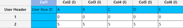
In the input datasheet minimum requirement is to specify one factor (column) and insert minimum two levels (values) for each factor (column), as shown below.
Configuration
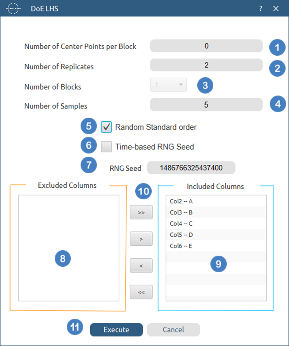
- Select
DOE\(\rightarrow\)Space Filling\(\rightarrow\)LHS. - Select the
Number of Center Points per Block[1] to be generated in the output list of experiments. - Select the
Number of Replicates[2]. The lowest value that can be set is 1. - Select the
Number of Blocks[3]. - Select the
Number of Samples[4] to be included in the output list of experiments. The lowest value that can get is 1. - Select/tick if required the
Random Standard order[5] to imply randomness in the output list of experiments. - If randomness is selected either select/tick to generate the number seed for randomness based on time [6] or by manually setting a value [7].
- Select the columns by clicking on the arrow buttons [10] and moving columns between the
Excluded Columns[8] andIncluded Columns[9] lists. - Click on the
Executebutton [11] to perform the LHS design method.
Output
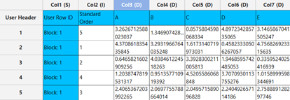
A list of experiments (combinations) is generated in the output datasheet along with the Block number based on the LHS method selected. Standard Order, Block number, Replicate Number and Point Type are presented in Cols 2,3,4 and 5 accordingly as shown below.
LHS Space Filling
Space-Filling Latin Hypercube Sampling (LHS) is an extension of the traditional Latin Hypercube Sampling method, designed to improve the uniformity of sample point distribution across the entire design space. While standard LHS ensures that each factor is uniformly sampled across its range by stratifying each dimension, Space-Filling LHS enhances this approach by striving to fill the design space as evenly as possible. This method avoids clustering of points and large gaps, providing more robust coverage in multidimensional spaces.
A key feature of Space-Filling LHS is its optimization of the placement of sample points to ensure a balance between points across all dimensions. While traditional LHS achieves one-dimensional uniformity, space-filling designs aim for multidimensional uniformity, ensuring that points are spread throughout the entire 𝑘-dimensional design space, reducing regions of high point density and minimizing large empty regions.
To achieve this the design aims to maximize the minimum distance between sample points, also referred to as “maximin” designs. Therefore, the distance between two points is as large as possible. Several optimization techniques can be applied to LHS to achieve this, such as minimizing a distance criterion or using evolutionary algorithms to adjust the positions of the sample points.
Given an $n × k$ Latin Hypercube $L = (l_{ij})$, a Space-Filling Latin hypercube design $D$ in the design space $[a_1, b_1] \times \cdots \times [a_k, b_k]$ ($[a_j, b_j]$ is the range of the $j^{th}$ factor) can be generated similarly to the standard LHS design, and the design matrix of $D$ is an $n × k$ matrix with the $(i, j)^{th}$ entry being:
where $u_{ij}$’s are independent random numbers from $[a_j, b_j]$ used to optimize the positions of the sampling points for better space-filling properties. The result is a design where points are more uniformly distributed across the entire multidimensional space.
The primary advantage of Space-Filling LHS over traditional LHS is its improved coverage of the design space in multiple dimensions. Traditional LHS provides one-dimensional uniformity by ensuring that each factor is sampled evenly across its range. However, this can sometimes result in points clustering together in certain regions of the space, particularly in high-dimensional settings. Space-Filling LHS reduces these clusters and ensures that the points are not only well distributed across each dimension but also across the full multidimensional space.
Space-Filling LHS is particularly valuable in cases where computational or experimental costs are high, and a limited number of samples must provide comprehensive coverage of the space. By ensuring that the sample points are spread evenly across the design space, Space-Filling LHS minimizes the number of samples needed while maintaining robust coverage.
Use the Space – Filling LHS designs by browsing in the top ribbon:
| DOE \(\rightarrow\) Space Filling \(\rightarrow\) LHS Space Filling |
Input
Numerical values should be specified in the input datasheet. Space-Filling LHS is applied when at least one factor (column) is specified along with at least two levels/values (rows) LHS will assume the lowest of the levels as the lower bound of the factor’s range and the highest of the levels as the higher bound of the factor’s range.
Configuration
| Number of Center Points per Block | Select manually the Number of Center Points per Block to be included in the output list of experiments. There is no minimum requirement or any other limitation. |
| Number of Replicates | Select manually the Number of Replicates which represents the number of times to replicate the entire design. This value should be an integer, and the lowest acceptable value is 1. |
| Number of Blocks | Select from the list of available options the Number of Blocks. These designs can only be blocked on replicates, so the available options include 1 and the selected Number of Replicates. |
| Number of Samples | Select manually the Number of Samples to be included in the output list of experiments. The lowest value that can get is 1. |
| Random Standard order | You can tick/select the box if randomness is required in the output list of experiments. |
| Time-based RNG Seed | If randomness is selected, then you have the option to also tick/select the box to set the random generated number seed based on time. |
| RNG Seed | Select manually the random generated number seed if required. |
| Include/exclude columns | Select manually the columns through the dialog window: Use the buttons to move columns between the Included Columns and Excluded Columns list. Single-arrow buttons will move all selected columns and double-arrow buttons will move all columns. |
Output
A list of experiments (combinations) is generated in the output datasheet along with the Block number, the Replicate Number, the Standard order and the Point type of each experiment based on the Space – Filling LHS design.
Example
Input
In the input datasheet minimum requirement is to specify one factor (column) and insert minimum two levels (values) for each factor (column), as shown below.

Configuration
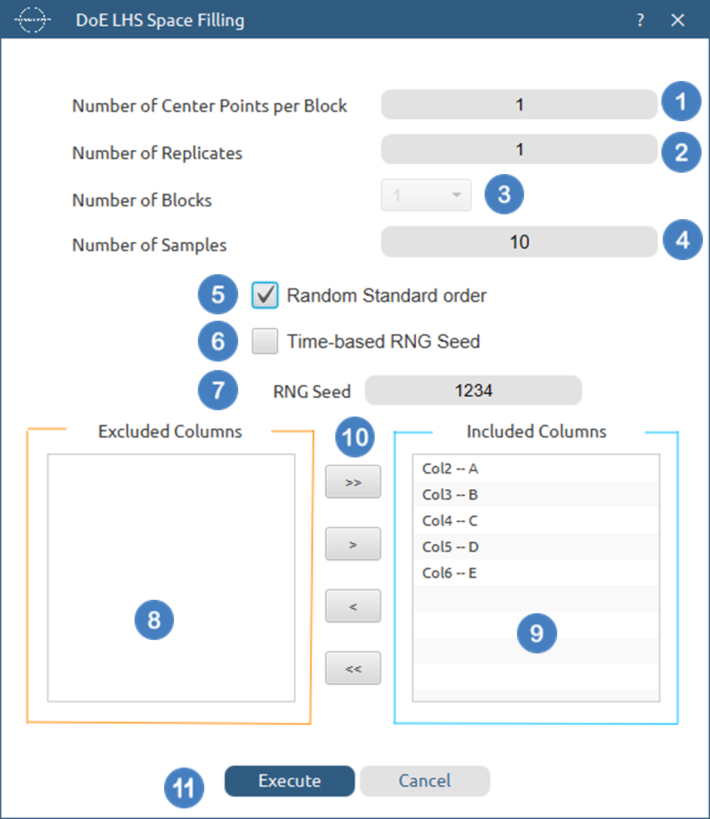
- Select
DOE\(\rightarrow\)Space Filling\(\rightarrow\)LHS Space Filling. - Select the
Number of Center Points per Block[1] to be generated in the output list of experiments. - Select the
Number of Replicates[2]. The lowest value that can be set is 1. - Select the
Number of Blocks[3]. - Select the
Number of Samples[4] to be included in the output list of experiments. The lowest value that can get is 1. - Select/tick if required the Random Standard order [5] to imply randomness in the output list of experiments.
- If randomness is selected either select/tick to generate the number seed for randomness based on time [6] or by manually setting a value [7].
- Select the columns by clicking on the arrow buttons [10] and moving columns between the
Excluded Columns[8] andIncluded Columns[9] lists. - Click on the
Executebutton [11] to perform the Space Filling LHS design method.
Output
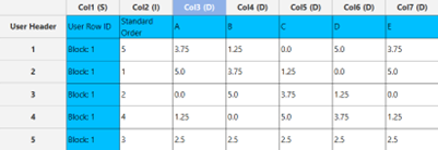
A list of experiments (combinations) is generated in the output datasheet along with the Block number based on the Space - Filling LHS method selected. Standard Order, Block number, Replicate Number and Point Type are presented in Cols 2,3,4 and 5 accordingly as shown below.
Sukharev Grid
The Sukharev Grid is part of a group of point dispersion approaches called low-dispersion sampling , which aims to minimize the largest uncovered space between sample points. Dispersion refers to the size of the largest gap or region between sampled points, and the goal of low-dispersion sampling is to reduce this gap to ensure more uniform coverage of the design space. By minimizing the dispersion, the Sukharev Grid forces sample points to be evenly distributed, avoiding clusters or large unrepresented regions in the design space.
When dispersion is minimized using the $L_\infty$ metric (the maximum norm, which measures the largest absolute difference between any two points), the result is a Sukharev Grid. The $L_\infty$ metric emphasizes the importance of covering the space evenly by prioritizing the minimization of the largest gap between any two sample points in a multidimensional grid.
To generate a Sukharev Grid, the design space is divided into a set of equally sized hypercubes (or “cubes” in lower dimensions). This partitioning is based on the number of factors $𝑛$, the number of sample points $𝑘$, and the range of each factor $[a_i, b_i]$. Each factor’s range is divided into $𝑘$ equal segments, and the grid points are placed at the center of each resulting hypercube.
Steps for constructing a Sukharev Grid:
- Divide each factor’s range $[a_i, b_i]$ into $𝑘$ equal segments, where $𝑘$ is the desired number of samples.
- Place points at the center of each hypercube formed by the partitioning of the space. The center is chosen because it minimizes the dispersion for each hypercube, ensuring that the points are as far as possible from the boundaries of the cubes.
- Mathematically, if the range of factor $𝑖$ is $[a_i, b_i]$, and we divide this range into $𝑘$ intervals, the center of each interval is located at: $c_{ij} = a_i + \left( j + \frac{1}{2} \right) \frac{(b_i - a_i)}{k}, \quad \text{for } j = 0, 1, 2, \dots, k-1$. The grid points for the design are the Cartesian products of the centers across all factors, ensuring that the points are evenly distributed throughout the design space.
The Sukharev Grid is particularly useful in situations where it is important to have uniform coverage of the design space with minimal computational cost. By optimizing dispersion, this grid ensures that no large regions are left unsampled, which is essential for applications requiring a thorough exploration of the design space.
The Sukharev Grid belongs to the family of low-discrepancy and low-dispersion methods, such as Halton sequences, and Latin Hypercube Sampling (LHS). While methods like Halton and sequences focus on generating quasi-random points with low discrepancy (a measure of how evenly points are distributed), the Sukharev Grid optimizes dispersion by minimizing the largest uncovered area in the space.
Use the Sukharev Grid design function by browsing in the top ribbon:
| DOE \(\rightarrow\) Space Filling \(\rightarrow\) Sukharev Grid |
Input
Numerical values should be specified in the input datasheet. Sukharev grid is applied when at least one factor (column) is specified along with at least two levels/values (rows). The method will assume the lowest of the levels as the lower bound of the factor’s range and the highest of the levels as the higher bound of the factor’s range.
Configuration
| Number of Center Points per Block | Select manually the Number of Center Points per Block to be included in the output list of experiments. There is no minimum requirement or any other limitation. |
| Number of Replicates | Select manually the Number of Replicates which represents the number of times to replicate the entire design. This value should be an integer, and the lowest acceptable value is 1. |
| Number of Blocks | Select from the list of available options the Number of Blocks. These designs can only be blocked on replicates, so the available options include 1 and the selected Number of Replicates. |
| Random Standard order | You can tick/select the box if randomness is required in the output list of experiments. |
| Time-based RNG Seed | If the randomness is selected, then you have the option to also tick/select the box to set the random generated number seed based on time. |
| RNG Seed | Select manually the random generated number seed if required. |
| Include/exclude columns | Select manually the columns through the dialog window: Use the buttons to move columns between the Included Columns and Excluded Columns list. Single-arrow buttons will move all selected columns and double-arrow buttons will move all columns. |
| Number of Samples | Select from the list provided the Number of Samples to be included in the output list of experiments. The available options range through $2^k$ to $9^k$, where $k$ is the number of included columns. |
Output
A list of experiments (combinations) is generated in the output datasheet along with the Block number, the Replicate Number, the Standard order and the Point type of each experiment based on the Sukharev Grid design method selected.
Example
Input
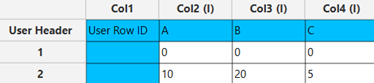
In the input datasheet minimum requirement is to specify three factors (columns) and insert minimum two levels (values) for each factor (column), as shown below.
Configuration
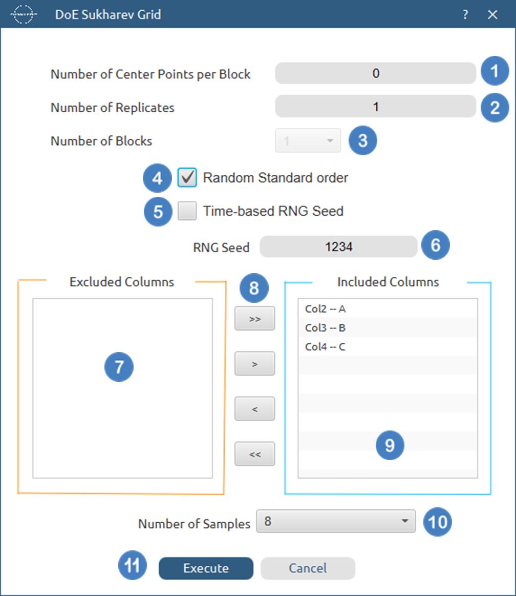
- Select
DOE\(\rightarrow\)Space Filling\(\rightarrow\)Sukharev Grid. - Select the
Number of Center Points per Block[1] to be generated in the output list of experiments. - Select the
Number of Replicates[2]. The lowest value that can be set is 1. - Select the
Number of Blocks[3]. - Select/tick if required the
Random Standard order[4] to imply randomness in the output list of experiments. - If randomness is selected either select/tick to generate the number seed for randomness based on time [5] or by manually setting a value [6].
- Select the columns by clicking on the arrow buttons [89 and moving columns between the
Excluded Columns[7] andIncluded Columns[8] lists. - Select the
Number of Samples[10] to be generated in the output list of experiments by selecting the desired number for the options provided in the list ($2^k$ to $9^k$, where $k$ is the number of included columns). - Click on the
Executebutton [11] to perform Sukharev Grid method.
Output
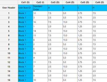
A list of 16 experiments (combinations) is generated in the output datasheet along with the Block number based on the Sukharev Grid method selected. Standard Order, Block number, Replicate Number and Point Type are presented in Cols 2,3,4 and 5 accordingly as shown below.
Uniform Design
A Uniform Design is a space-filling design of experiments (DoE) method that places runs so the design points are distributed as evenly as possible throughout the experimental region. The objective is global coverage: avoiding clusters and leaving as few “holes” in the design space as possible. This is particularly useful when:
- the response surface is unknown or potentially nonlinear,
- interaction and curvature may exist,
- each run is expensive (e.g., simulations, prototypes), and
- you want broad exploration rather than local refinement.
To make even coverage measurable, Uniform Design uses a quantitative uniformity metric. In this implementation, Centered \(L_2\) discrepancy is used to evaluate how closely the point set resembles a uniform distribution over the unit hypercube. The design is generated to minimize this discrepancy (smaller values indicate a more uniform point set).
Centered \(L_2\) discrepancy
Let \(P_n=\{x_1,…,x_n\}\) be the set of ndesign points in sdimensions, with coordinates \(x_{kj} ∈ [0,1]\)(i.e., factor levels scaled to the unit interval). The squared centered \(L_2\) discrepancy is:
where,
- n= number of runs (design points)
- s= number of factors (dimensions)
- \(x_{kj}\)= value of factor j in run k, scaled to \([0,1]\)
The best design is obtained by a two-stage optimization procedure. Firstly, the Threshold Accepting algorithm is used to generate a strong initial discretized design. The result is then refined in the continuous design space using Coordinate Descent, which improves uniformity by iteratively adjusting coordinates to further reduce the centered \(L_2\) discrepancy.
This combination provides both exploration (global search via Threshold Accepting) and polishing (local improvement via Coordinate Descent). Use the Uniform Design function by browsing in the top ribbon:
| DOE \(\rightarrow\) Space Filling \(\rightarrow\) Uniform |
Input
In the input data sheet, specify at least two numerical columns. Each factor column must contain at least two non-empty cells. Isalos sets Low = minimum and High = maximum of the provided values and sets the Center level to (Low + High)/2.
Configuration
| Number of Center Points per Block | Select manually the Number of Center Points per Block to be included in the output list of experiments. There is no minimum requirement or any other limitation. |
| Number of Replicates | Select manually the Number of Replicates which represents the number of times to replicate the entire design. This value should be an integer, and the lowest acceptable value is 1. |
| Number of Blocks | Select from the list of available options the Number of Blocks. These designs can only be blocked on replicates, so the available options include 1 and the selected Number of Replicates. |
| Number of Samples | Select manually the Number of Samples to be included in the resulting design. The lowest value it can get is 1. |
| Random Standard order | You can tick/select the box if randomness is required in the output list of experiments. |
| Time-based RNG Seed | If in the randomness is selected, then you have the option to also tick/select the box to set the random generated number seed based on time. |
| RNG Seed | Select manually the random generated number seed if required. |
| Include/exclude columns | Select manually the columns through the dialog window: Use the buttons to move columns between the Included Columns and Excluded Columns list. Single-arrow buttons will move all selected columns and double-arrow buttons will move all columns. |
Output
A list of experiments (combinations) is generated in the output datasheet along with the Block number, the Replicate Number, the Standard order and the Point type of each experiment based on the Uniform Design method. Next to the design table the squared centered L2 discrepancy for the selected points is shown.
Example
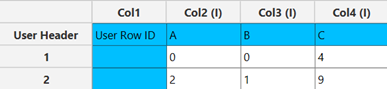
Input
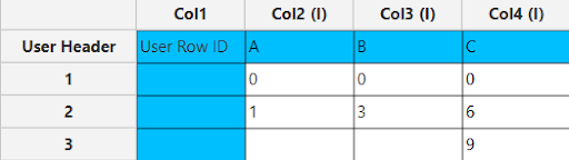
In the input datasheet minimum requirement is to specify three factors (columns) and insert minimum two levels (values) for each factor (column), as shown below.
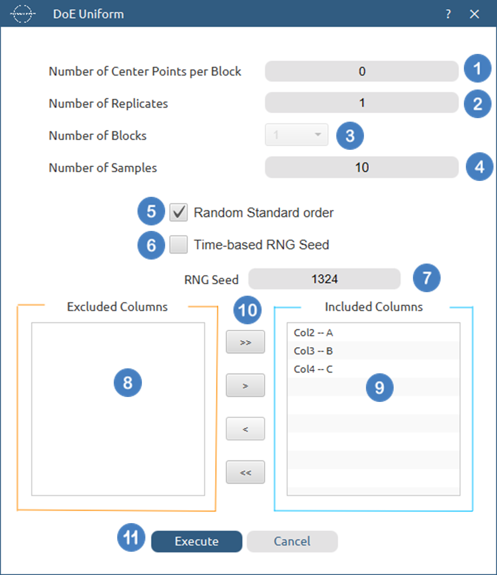
Configuration
- Select
DOE\(\rightarrow\)Space Filling\(\rightarrow\)Uniform. - Select the
Number of Center Points per Block[1] to be generated in the output list of experiments. - Select the
Number of Replicates[2]. The lowest value that can be set is 1. - Select the
Number of Blocks[3]. - Select the
Number of Samples[4] to be generated. The lowest value that can be set is 1. - Select/tick if required the
Random Standard order[5] to imply randomness in the output list of experiments. - If randomness is selected either select/tick to generate the number seed for randomness based on time [6] or by manually setting a value [7].
- Select the columns by clicking on the arrow buttons [10] and moving columns between the
Excluded Columns[8] andIncluded Columns[9] lists. - Click on the
Executebutton [11] to perform the Uniform design method.
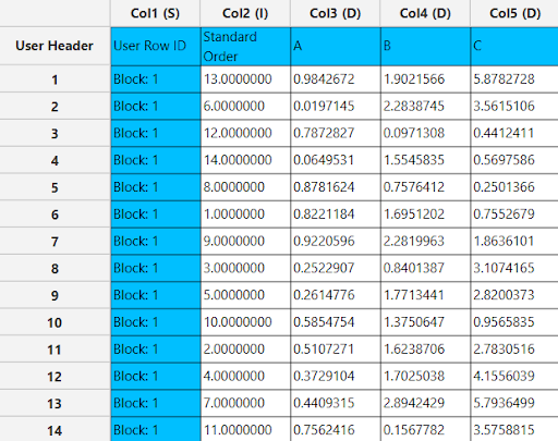
Output
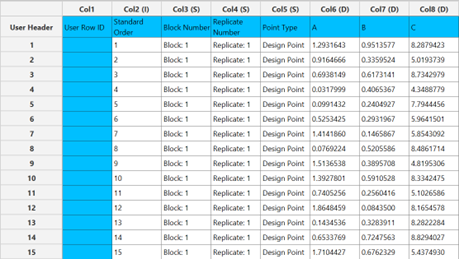
The output list of experiments is generated for the three factors outlining a list of 15 experiments based on the Definitive Screening design. Standard Order, Block number, Replicate Number and Point Type are presented in Cols 2,3,4 and 5 accordingly as shown below. The Squared Centered L2 Discrepancy for the selected points is 0.0035895
Monte-Carlo Sampling
Monte Carlo Sampling is a simple and widely used space-filling approach that generates design points by randomly sampling each factor from a specified probability distribution, most commonly the uniform distribution over the factor range. The objective is to obtain a representative spread of points across the design space, so the resulting data supports exploration of the relationship between the input factors and the response variable.
Unlike structured space-filling designs (e.g., uniform or low-discrepancy designs), Monte Carlo Sampling does not explicitly enforce even spacing. As a result, points may form clusters or leave gaps, especially when the number of samples is small or the number of factors is large. However, Monte Carlo Sampling is often attractive because it is:
- Straightforward to generate and scale to any number of factors,
- Flexible, supporting arbitrary ranges ,
- Computationally inexpensive, and
- Easy to increase incrementally (additional samples can be appended without redesign).
To construct a Monte Carlo sample in Isalos, a random seed is specified to ensure reproducibility. For a design with s factors and n samples, we generate n values for each factor by sampling from a uniform distribution on (0,1). The sampled values are then linearly scaled to each factor’s specified range to obtain points in the original design space.
This procedure is efficient, easy to implement, and provides a practical baseline sampling method when a fully optimized space-filling design is not required.
Use the Monte-Carlo Sampling function by browsing in the top ribbon:
| DOE \(\rightarrow\) Space Filling \(\rightarrow\) Monte-Carlo Sampling |
Input
In the input data sheet, specify at least two numerical columns. Each factor column must contain at least two non-empty cells. Isalos sets Low = minimum and High = maximum of the provided values and sets the Center level to (Low + High)/2.
Configuration
| Number of Center Points per Block | Select manually the Number of Center Points per Block to be included in the output list of experiments. There is no minimum requirement or any other limitation. |
| Number of Replicates | Select manually the Number of Replicates which represents the number of times to replicate the entire design. This value should be an integer, and the lowest acceptable value is 1. |
| Number of Blocks | Select from the list of available options the Number of Blocks. These designs can only be blocked on replicates, so the available options include 1 and the selected Number of Replicates. |
| Number of Samples | Select manually the Number of Samples to be included in the resulting design. The lowest value it can get is 1. |
| Random Standard order | You can tick/select the box if randomness is required in the output list of experiments. |
| Time-based RNG Seed | If in the randomness is selected, then you have the option to also tick/select the box to set the random generated number seed based on time. |
| RNG Seed | Select manually the random generated number seed if required. |
| Include/exclude columns | Select manually the columns through the dialog window: Use the buttons to move columns between the Included Columns and Excluded Columns list. Single-arrow buttons will move all selected columns and double-arrow buttons will move all columns. |
Output
A list of experiments (combinations) is generated in the output datasheet along with the Block number, the Replicate Number, the Standard order and the Point type of each experiment based on the Uniform Design method.
Example
Input
In the input datasheet minimum requirement is to specify three factors (columns) and insert minimum two levels (values) for each factor (column), as shown below.
Configuration
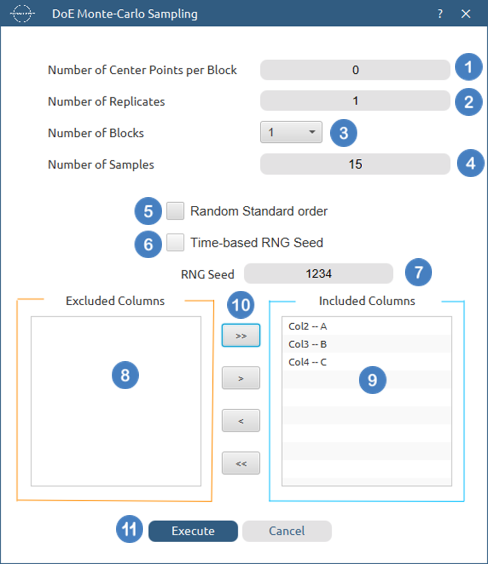
- Select
DOE\(\rightarrow\)Space Filling\(\rightarrow\)Monte-Carlo Sampling. - Select the
Number of Center Points per Block[1] to be generated in the output list of experiments. - Select the
Number of Replicates[2]. The lowest value that can be set is 1. - Select the
Number of Blocks[3]. - Select the
Number of Samples[4] to be generated. The lowest value that can be set is 1. - Select/tick if required the
Random Standard order[5] to imply randomness in the output list of experiments. - If randomness is selected either select/tick to generate the number seed for randomness based on time [6] or by manually setting a value [7].
- Select the columns by clicking on the arrow buttons [10] and moving columns between the
Excluded Columns[8] andIncluded Columns[9] lists. - Click on the
Executebutton [11] to perform the Monte-Carlo Sampling design method.
Output
The output list of experiments is generated for the three factors outlining a list of 15 experiments based on the Definitive Screening design. Standard Order, Block number, Replicate Number and Point Type are presented in Cols 2,3,4 and 5 accordingly as shown below.
References
-
Box, G.E. and Behnken, D.W., Some new three level designs for the study of quantitative variables. Technometrics, 1960. 2(4): p. 455-475. doi.org/10.1080/00401706.1960.10489912.
-
Box, G.E. and Wilson, K.B., On the experimental attainment of optimum conditions, in Breakthroughs in statistics: methodology and distribution. 1992, Springer. p. 270-310. doi.org/10.1007/978-1-4612-4380-9_23.
-
Montgomery, Douglas C. Design and analysis of experiments. John wiley & sons, 2017.
-
Speed, Terry. Statistics for Experimenters: Design, Innovation, and Discovery. 2006.
-
Wu, CF Jeff, and Michael S. Hamada. Experiments: planning, analysis, and optimization. John Wiley & Sons, 2011.
-
Lai, Jianfa, Kai-Tai Fang, Xiaoling Peng, and Yuxuan Lin. “Construction of uniform designs over continuous domain in computer experiments.” Communications in Statistics-Simulation and Computation 53, no. 1 (2024): 130-146.
-
Morris, Max D., and Toby J. Mitchell. “Exploratory designs for computational experiments.” Journal of statistical planning and inference 43, no. 3 (1995): 381-402.
-
Joseph, V. Roshan. “Space-filling designs for computer experiments: A review.” Quality Engineering 28, no. 1 (2016): 28-35.
-
Fang, Kai-Tai, Dennis KJ Lin, Peter Winker, and Yong Zhang. “Uniform design: theory and application.” Technometrics 42, no. 3 (2000): 237-248.
Version History
Introduced in Isalos Analytics Platform v0.2.4
Instructions last updated on November 2025