Classification
Classification is a typical supervised learning technique in predictive modeling that aims to categorize data into predefined classes. Classification analysis is used when the target is a categorical value, and algorithms are trained on labeled datasets to predict the category of unseen objects. There are two types of classification problems; Binary classification where the possible outcome can be one of two distinct classes, and Multiclass classification where the outcome can be one of several categories. 1
k Nearest Neighbors (kNN)
k Nearest Neighbors (kNN) is a simple non-parametric algorithm that operates by identifying the data points from the training set that are most proximate to a new unseen input. This instance-based learning method calculates the Euclidean distance between instances considering all attribute values in order to determine the closeness between data points. The k parameter denotes the number of nearest neighbors to consider for the prediction.1,2 The prediction of a new instance is assigned based on the class label that is most frequently represented among the k nearest neighbors using the inverted distance as the weighting factor. As calculations of Euclidean distances are performed, scaling of data is performed within the function.
Use the k Nearest Neighbors classification function by browsing in the top ribbon:
| Analytics \(\rightarrow\) Classification \(\rightarrow\) k Nearest Neighbors (kNN) |
Input
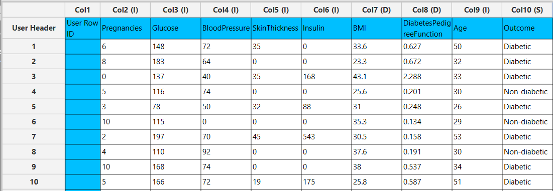
Data matrix with training set data. The categories of the target feature should be presented as strings.
Configuration
| Target Column | Select from the drop-down menu the column containing the target (dependent) variable that is going to be predicted. Columns with numerical features cannot be selected as targets. |
| Number of Neighbors | An integer representing the number of closest data points (k) used to make predictions for a new data point. |
Output
A data matrix including the actual target value and the value predicted by the algorithm (“kNN Prediction”). For each data point, the closest neighbors from the training set are listed in the “Closest NN” columns, along with their corresponding distances in the “Distance from NN” columns.
Example
Input
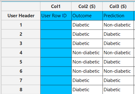
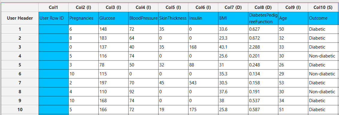
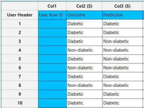
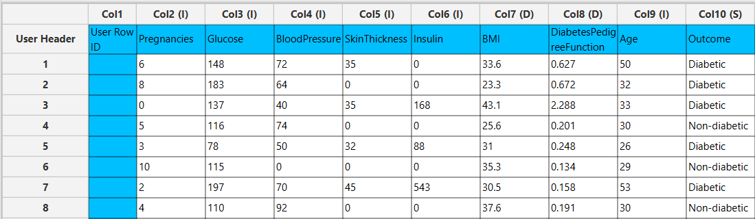
In the left-hand spreadsheet of the tab import the data matrix including the target variable for prediction.
Configuration
- Select
Analytics\(\rightarrow\)Classification\(\rightarrow\)k Nearest Neighbors (kNN). - Select the column that is going to be predicted from the drop-down menu [1].
- Type the
Number of Neighbors[2] to consider. - Click on the
Executebutton [3] to apply the training algorithm on the input columns.

Output
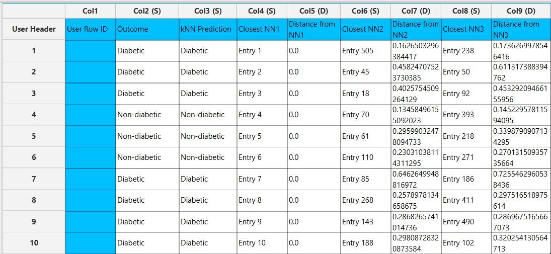
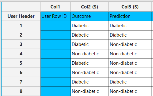
In the right-hand spreadsheet of the tab the output data matrix with the actual and the predicted value of the target is presented. Also, the k most proximate identified instances from the training set are given for each data point, along with the corresponding inverted Euclidean distances from each neighbor. Note that the “Closest NN1” represents the nearest neighbor, which is the data point itself when applied on the training set. Consequently, the “Distance from NN1” is 0 for all given training instances.
Application on external set
You can apply the trained k Nearest Neighbors (kNN) model to any external (test) data using the Existing Model Utilization function:
- Import the external data in the left-hand spreadsheet of the tab. Include the same columns used to build the kNN model.
- Select
Analytics\(\rightarrow\)Existing Model Utilization. Select the kNN model [1] and click on theExecutebutton [2].

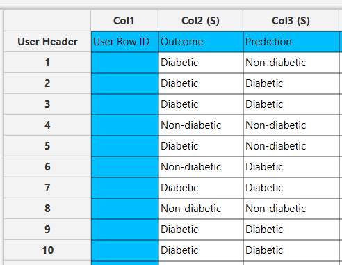
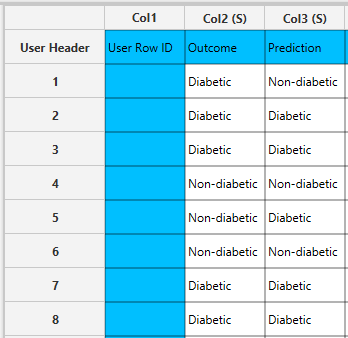
- Inspect the results in the right-hand spreadsheet of the tab. Note that in this case the closest neighbor listed in the “Closest NN1” belongs to the training set, and the “Distance from NN1” is not zero.

Fully Connected Neural Network
A type of feedforward artificial neural network consisting of multiple layers of neurons. It consists of an input layer, one or more hidden layers and an outer layer, which are fully connected with each other. A variety of non-linear activation functions are typically used in the hidden layer, allowing the network to learn complex patterns in data. MLP uses a backpropagation algorithm to train the model and classify instances.1,2
Use the Fully Connected Neural Network function by browsing in the top ribbon:
| Analytics \(\rightarrow\) Classification \(\rightarrow\) Fully Connected Neural Network |
Input
Data matrix with training set data. The categories of the target feature should be presented as strings. Other categorical features must be encoded into numerical values, presented as either integers or doubles.
Configuration
| Batch Size | Select from the drop-down menu the number of training instances that will be propagated through the network. Four options are available for selection: 16, 32, 64, and 128. |
| Number of Epochs | Specify the number (integer) of complete passes through the data during training. |
| Learning Rate | Specify the learning rate (between 0 and 1), which controls the size of the steps taken during optimization. |
| Momentum | Specify the momentum rate (between 0 and 1) for the backpropagation algorithm. |
| +/- | Click on the + and - buttons to add or remove hidden layers, respectively. |
| Hidden Layers | For each added hidden layer, specify the number of neurons and select the non-linear activation function used to map the weighted inputs to the output of each neuron. Options for the activation functions include: - RELU, - RELU6, - LEAKYRELU, - SELU, - SWISH, - RRELU, - SIGMOID, - SOFTMAX, - SOFTPLUS, - SOFTSIGN, - TANH, - THRESHOLDEDRELU, - GELU, - ELU, - MISH, - CUBE, - HARDSIGMOID, - HARDTANH, - IDENTITY, - RATIONALTANH, and - RECTIFIEDTANH. |
| Target Column | Select from the drop-down menu the column containing the feature that is going to be predicted. |
| RNG Seed | Select an integer as seed to get reproducible results. The option to select a time-based random number-generated seed is available. |
Output
A data matrix including the actual categorical value and the class predicted by the algorithm (“Prediction”) is presented.
Example
Input
In the left-hand spreadsheet of the tab import the data matrix including the target variable with at least two distinct categories for prediction. In case that categorical-string columns are included in the set, these should be encoded into representative numerical values.

Configuration
- Select
Analytics\(\rightarrow\)Classification\(\rightarrow\)Fully Connected Neural Network - Select the hyperparameters that determine the training procedure: the
Batch Size[1], theNumber of Epochs[2], theLearning Rate[3] and theMomentum[4]. - Select the hyperparameters that determine the
Hidden Layers[5] of the neural network: the number of neurons [6] and the activation function [7] of each layer. - Add [8] or remove [9] hidden layers to define the architecture of the neural network.
- Select the column that is going to be predicted from the drop-down menu [10]. Only columns containing categorical features should be selected for prediction.
- Select an
RNG Seedfor reproducible results or a random number generatedTime-based (RNG) Seed[11]. - Click on the
Executebutton [12] to apply the training algorithm on the input columns.

Output
In the right-hand spreadsheet of the tab the output data matrix with the actual and the predicted category of the target is presented.
Radial Basis Function Network
Radial basis function networks (RBF) network is an artificial neural network that employs RBF kernels as activation functions. The network consists of three layers: the input layer modeling a vector that passes data, the hidden layer that performs computations and the output layer designated for classification problems. The output layer of the neural network is a linear combination of the activation (output) from the hidden units.5,6
A Radial Basis Function is a real-valued function $φ(r)$ that is dependent only on the distance between a fixed input point ($r$) to the center ($c$) of each neuron as reference point Eq. 1.3
The radial basis function kernels available in Isalos include:
Gaussian:
Multiquadric:
Inverse Quadratic:
Inverse Multiquadric:
Polyharmonic spline:
where $k$ is the order of the spline.
Thin Plate Spline:
Bump Function:
where $\varepsilon$ is the shape parameter used to scale the input of the radial kernel.
Use the Radial Basis Function Network classification function by browsing in the top ribbon:
| Analytics \(\rightarrow\) Classification \(\rightarrow\) Radial Basis Function Network |
Input
Data matrix with training set data. The categories of the target feature should be presented as strings. Other categorical features must be encoded into numerical values, presented as doubles, since RBF does not allow the use of integers.
Configuration
| Hidden Neurons | Specify the number of neurons in the hidden layer of the network. |
| RBF Kernel | Select from the drop-down menu the radial basis function kernel. Options include: - GAUSSIAN Eq. 2, - MULTIQUADRIC Eq. 3, - INVERSE QUADRATIC Eq. 4, - INVERSE MULTIQUADRIC Eq. 5, - POLYHARMONIC SPLINE Eq. 6, - THIN PLATE SPLINE Eq. 7, and - BUMP FUNCTION Eq. 8. A new configuration field appears accordingly after RBF Kernel selection, for the selection of Epsilon ($\varepsilon$) shape parameter or K ($k$) where applicable. |
| Point Selection | Select manually the way that determines how the centers of the neural network are chosen. Options include: - Random Points from Training set: chosen randomly from the training data. - Use KMeans: RBF centers are the cluster centers of the partitioned training data. |
| RNG Seed | Select an integer as seed to get reproducible results. The option to select a time-based random number-generated seed is available. |
| Target Column | Select from the drop-down menu the column containing the target variable that is going to be predicted. Columns with numerical features cannot be selected as targets. |
Output
A data matrix including the actual categorical value and the class predicted by the algorithm (“Prediction”) is presented.
Example
Input
In the left-hand spreadsheet of the tab import the data matrix including the target variable for prediction containing at least two distinct categories presented as strings. In case that categorical-string columns are included in the set, these should be encoded into representative numerical values (doubles).
- Select
Analytics\(\rightarrow\)Classification\(\rightarrow\)Radial Basis Function Network - Type the number (integer) of
Hidden Neurons[1]. - Select the
RBF Kernel[2] used as activation function of the hidden layer and subsequently select theEpsilon[3] orKparameter where applicable. - Select the
Point Selection[4] method to determine the center of the network. - Select an
RNG Seedfor reproducible results or a random number generatedTime-based (RNG) Seed[5]. - Select the column that is going to be predicted from the drop-down menu [6].
- Click on the
Executebutton [7] to apply the normalization on the selected columns.

Output
In the right-hand spreadsheet of the tab the output data matrix with the actual and the predicted category of the target is presented.
XGBoost
The Extreme Gradient Boosting (XGBoost) open-source library7 is used to implement the gradient boosting framework. The library uses a class of ensemble machine learning algorithms constructed from decision tree models. Ensemble learning operates by combining different individual base learners to obtain a final prediction.8 In an iterative process, trees are added to the ensemble so that the prediction error (loss) of previous models is reduced. In classification tasks, there are different loss functions available for binary and multiclass problems.9
Use the XGBoost classification function by browsing in the top ribbon:
| Analytics \(\rightarrow\) Classification \(\rightarrow\) XGBoost |
Input
Data matrix with training set data. The categories of the target feature should be presented as strings. Other categorical features must be encoded into numerical values, presented as doubles.
Configuration
| Target Column | Select from the drop-down menu the column containing the target variable that is going to be predicted. Columns with numerical features cannot be selected as targets. |
| booster | Select from the drop-down menu which booster to use. Three options are available for selection, namely: - gbtree: default tree-based models, - dart: tree-based models, and - gblinear: linear functions. |
| objective | Select from the drop-down menu the learning objective of the method. Options include: - reg:squarederror: regression with squared loss, - reg:gamma: gamma regression with log-link, whose output is a mean of gamma distribution, and - reg:tweedie: tweedie regression with log-link. |
| number of estimators | Type the number of models (integer) to train in the learning ensemble. |
| eta | Specify the learning rate (between 0 and 1) which determines the step size shrinkage to prevent overfitting (default value: 0.3). |
| gamma | Specify the minimum loss reduction required to make a further partition on a leaf node of the tree (default value: 0). |
| max depth | Specify the maximum depth of a tree as a positive integer (default value: 6). |
| min child weight | Specify the minimum sum of instance weight (hessian) needed in a child (default value: 1). |
| column sample by tree | Specify the subsample ratio of features when constructing each tree. Subsampling will occur once for every tree constructed. |
| sub sample | Specify the subsampling ratio (between 0 and 1) of the training instances. Subsampling will occur once in every boosting iteration (default value: 1). |
| tree method | Select the tree construction algorithm used in XGBoost. Options include: - auto: use this heuristically to choose the fastest method typically based on the dataset size, - exact: exact greedy algorithm, - approx: approximates the greedy algorithm using quantile sketch and gradient histogram, and - hist: fast histogram optimized approximate greedy algorithm. |
| lambda | Specify the L2 regularization term on leaf weights (default value: 1). |
| alpha | Specify the L1 regularization term on leaf weights (default value: 0). |
| RNG Seed | Select an integer as seed to get reproducible results. The option to select a time-based random number-generated seed is available by clicking on the Time-based RNG Seed checkbox. |
Output
A data matrix including the actual categorical value and the class predicted by the algorithm (“Prediction”) is presented.
Example
Input
In the left-hand spreadsheet of the tab import the data matrix including the target variable for prediction containing at least two distinct categories presented as strings. In case that categorical-string columns are included in the set, these should be encoded into representative numerical values.
Configuration
- Select
Analytics\(\rightarrow\)Classification\(\rightarrow\)XGBoost. - Select the column that is going to be predicted from the drop-down menu [1].
- Select the tree
booster[2] method, theobjectivefunction [3] for loss and type thenumber of estimators[4] involved in the ensemble. - Select the hyperparameters involved in the regularization of the model:
eta[5],gamma[6],lambda[12] andalpha[13]. Select the hyperparameters involved in tree construction:max depth[7] andmin child weight[8]. Select the column sampling rate by tree [9] and the overall subsampling rates [10]. Default values, data types (double or integer) and acceptable ranges are indicated as guidance on the input parameter values. - Select the tree construction algorithm [11] used in the XGBoost.
- Select an
RNG Seedfor reproducible results or a random number generatedTime-based (RNG) Seed[14]. - Click on the
Executebutton [15] to apply the training algorithm on the input columns.

Output
In the right-hand spreadsheet of the tab the output data matrix with the actual and the predicted category of the target is presented.
J48 Decision Tree
J48 is an open-source Java implementation of the C4.5 statistical classifier, which performs classification based on pruned or unpruned decision trees or rules generated from them. In this interpretation, the algorithm uses the normalized information gain as criterion to split the dataset into subsets and uses the most influential attribute to make the decision in each node. J48 uses the pruning technique, which refers to the removal of branches from a decision tree that have limited contribution to the predictive performance of the model.1,10
Use the J48 Decision Tree classification function by browsing in the top ribbon:
| Analytics \(\rightarrow\) Classification \(\rightarrow\) J48 Decision Tree |
Input
Data matrix with training set data. The categories of the target feature should be presented as strings. Other categorical features must be encoded into numerical values, presented as either integers or doubles.
Configuration
| Minimum Sample Split | Specify the minimum number of data samples required to split a node. |
| Max Depth | Select the maximum depth in the decision tree. |
| Target Column | Select from the drop-down menu the column containing the feature that is going to be predicted. Columns with numerical features should not be selected as targets. |
Output
A data matrix including the actual categorical value and the class predicted by the algorithm (“Prediction”) is presented. The visualization of the constructed decision tree can be also generated.
Example
Input
In the left-hand spreadsheet of the tab import the data matrix including the target variable with at least two distinct categories for prediction. In case that categorical-string columns are included in the set, these should be encoded into representative numerical values.
Configuration
- Select
Analytics\(\rightarrow\)Classification\(\rightarrow\)J48 Decision Tree - Select the hyperparameters that determine the structure of the decision tree: the
Min sample split[1] andMax Depth[2]. Default values, data types and acceptable ranges are indicated as guidance on the input parameter values. - Select the column that is going to be predicted from the drop-down menu [3]. Only columns containing categorical features should be selected for prediction.
- Click on the
Executebutton [4] to apply the training algorithm on the input columns.

Output
In the right-hand spreadsheet of the tab the output data matrix with the actual and the predicted category of the target is presented.
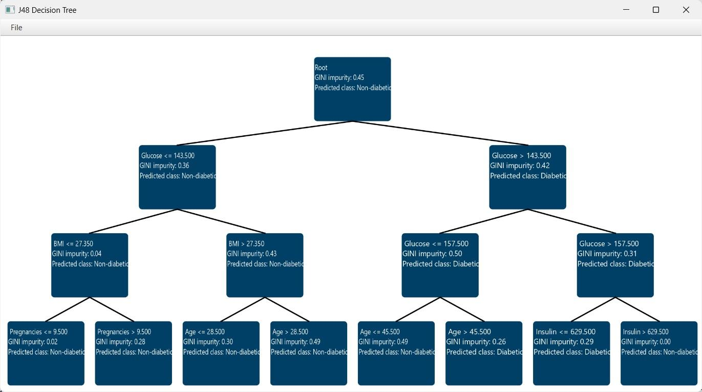
After the predictions are obtained, the option Draw Decision Tree [1] appears on the configuration window. Clicking this button will provide a visualization of the constructed decision tree.

The decision tree appears in a new window, offering a detailed view to help understand the decision-making process of the model. Specifically, each node is represented as a box containing information about the selected feature and its threshold used for data splitting. Also, the measured node purity (Gini) is presented, as well as the majority class that is predicted in each node.
Random Forest
Random forest classifier is an ensemble learning method that operates by building multiple randomized decision trees during training and obtaining the category prediction from each tree. The decision trees are constructed in parallel, with no interaction between them, using random subsets of training data and input attributes to ensure diversity. Classifications independently made by all the trees in the forest are aggregated and the majority vote is selected as the final class prediction.8,11
Use the Random Forest function by browsing in the top ribbon:
| Analytics \(\rightarrow\) Classification \(\rightarrow\) Random Forest |
Input
Data matrix with training set data. The categories of the target feature should be presented as strings. Other categorical features must be encoded into numerical values, presented as either integers or doubles.
Configuration
| Features fraction | Specify the feature subsampling rate represented as a fraction of features (between 0 and 1) available in each tree split (default value: 0.9). |
| Min impurity decrease | Specify the impurity decrease threshold (between 0 and 1) necessary to determine the quality of splits in the decision trees. A split is only considered if it results in a decrease of impurity greater than or equal to this value (default value: 0.1). |
| Seed | Select an integer as seed to get reproducible results. The option to select a time-based random number-generated seed is available. |
| Number of ensembles | Specify the number of individual trees to be generated by the algorithm (default value: 10). |
| Target column | Select from the drop-down menu the column containing the feature that is going to be predicted. Columns with numerical features cannot be selected as targets. |
Output
A data matrix including the actual categorical value and the class predicted by the algorithm (“Prediction”) is presented.
Example
Input
In the left-hand spreadsheet of the tab import the data matrix including the target variable for prediction with at least two distinct categories presented as strings. In case that other categorical-string features are included in the set, these should be encoded into representative numerical values.

Configuration
- Select
Analytics\(\rightarrow\)Classification\(\rightarrow\)Random Forest. - Select the hyperparameters that determine the structure of the model: the
Features fraction[1],Min impurity decrease[2] andNumber of ensembles[4]. Default values, data types (double or integer) and acceptable ranges are indicated as guidance on the input parameter values. - Select a
Seedfor reproducible results or a random number generatedTime-based (RNG) Seed[3]. - Select the column that is going to be predicted from the drop-down menu [5]. Only columns containing categorical features should be selected for prediction.
- Click on the
Executebutton [6] to apply the training algorithm on the input columns.

Output
In the right-hand spreadsheet of the tab the output data matrix with the actual and the predicted category of the target is presented.
Statistical fitting
Generalized Linear Models
Generalized Linear Models (GLMs) are a flexible class of regression and classification models that generalize ordinary linear regression to allow for response variables that have error distributions other than the normal distribution. GLMs are particularly useful when the response variable is categorical (e.g., binary outcomes) or count data, where assumptions of normality and constant variance are inappropriate. A GLM consists of three components:
- Random Component: The response variable \(y_i\) is assumed to follow a distribution from the exponential family (e.g., Normal, Binomial, Poisson, Gamma).
- Systematic Component: A linear predictor \(\eta_i= x_i^T \beta\), where \(x_i\) is the vector of predictors for the i-th observation, and \(\beta\) is the vector of coefficients.
- Link Function: A smooth, monotonic function \(g(⋅)\) that relates the mean \(\mu_i= E[y_i]\) of the response to the linear predictor via \(g(\mu_i )= \eta_i\).
Unlike traditional linear regression, GLMs do not assume a linear relationship between the predictors and the response. Instead, the link function transforms the expected value of the response variable to a scale where it can be modeled as a linear combination of the predictors. GLM parameters are estimated using Maximum Likelihood Estimation (MLE). The likelihood is constructed based on the assumed distribution of the response variable, and the log-likelihood function is maximized to obtain the parameter estimates. Because log-likelihood is usually a nonlinear function of the parameters, iterative optimization method such as Newton-Raphson and Fisher Scoring are used to obtain the maximum likelihood estimates of the parameters of each model. Categorical variables are encoded using one-hot encoding, where each category is represented by a binary (0 or 1) dummy variable. The reference category for each categorical variable is the first observed category, and its corresponding dummy variable is omitted to avoid multicollinearity. This omission allows the reference category to be implicitly represented in the model intercept, providing a baseline for interpreting the effects of the other categories.
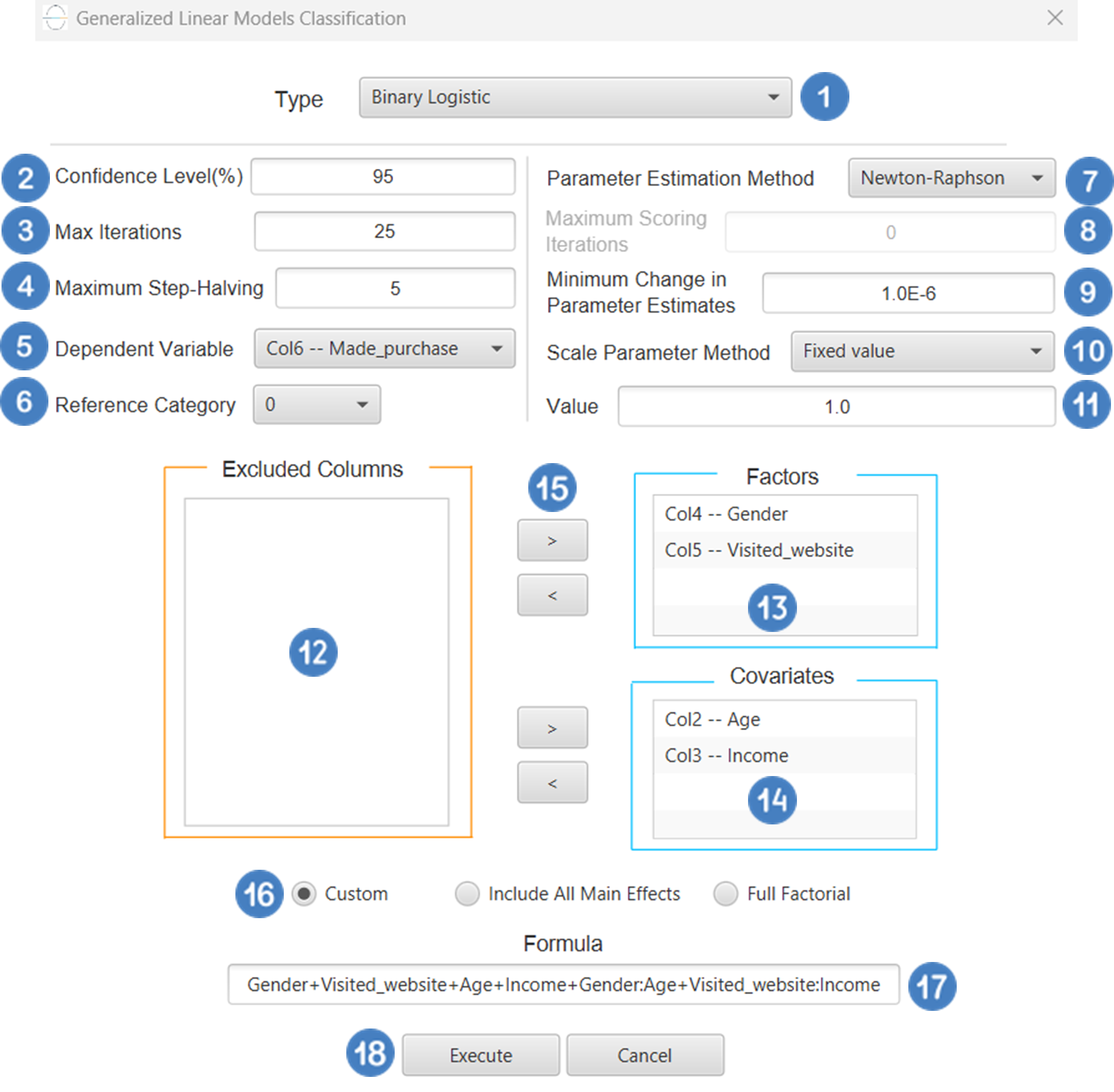
Binary Logistic
Binary Logistic Classification is a type of generalized linear model used when the dependent variable is binary, meaning it takes only two possible outcomes (e.g., success/failure, yes/no, 1/0). The response variable is assumed to follow a binomial distribution, where each observation represents a single Bernoulli trial. Unlike linear regression, logistic regression uses the logit link function, defined as:
Where \(\mu\) is the probability of the event occurring (i.e., the probability that the dependent variable equals 1). This transformation ensures that the predicted probabilities always fall within the [0,1] interval. Binary logistic classification is widely used in fields such as medicine, social sciences, marketing, and machine learning, particularly when the goal is to model and predict a binary outcome based on one or more predictor variables (either continuous or categorical).
Use the Binary Logistic Classification method by browsing in the top ribbon:
| Analytics \(\rightarrow\) Classification \(\rightarrow\) Statistical fitting \(\rightarrow\) Generalized Linear Models |
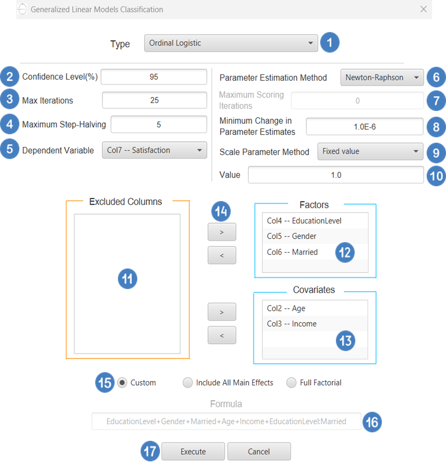
And then choosing “Binary Logistic” as the Type.
Input
All variables must be specified in the datasheet. Numerical values are required for covariates, while factors may be either textual or numerical. The dependent variable must be binary, typically coded as 0 and 1, representing the two possible outcome categories. The design for Binary Logistic Classification requires at least two columns in the input sheet: one column for the binary dependent variable and at least one column for an independent variable (either a categorical factor or a numerical covariate). Each row corresponds to a single observation.
Configuration
| Confidence Level (%) | Specify the confidence level of the analysis. Values should range from 0 to 100 and correspond to percentages. |
| Max Iterations | Defines the maximum number of iterations the model is allowed to perform during the estimation process. If the model fails to converge before reaching this number, the algorithm stops and returns the values of the last iteration. |
| Maximum Step-Halving | Controls how many times the algorithm is allowed to halve the step size during parameter updates when an iteration leads to worse model fit. |
| Dependent Variable | Select the column that corresponds to values of the dependent variable. |
| Reference Category | Specifies which category of the dependent variable should be used as the reference level when calculating parameter estimates. |
| Parameter Estimation | This option lets you choose how the model parameters will be estimated, Newton-Raphson, Fisher Scoring or Hybrid. |
| Maximum Scoring Iterations | The “Maximum Scoring Iterations” parameter is used when the hybrid estimation method is selected, instead of Newton-Raphson or Fisher scoring alone, and specifies the maximum number of iterations to be performed during the scoring phase. |
| Minimum Change in Parameter Estimates | Sets the tolerance level for convergence — the smallest change in parameter estimates between iterations required to continue optimization. If the change in all parameters is below this value, the algorithm assumes convergence has been reached. |
| Scale Parameter Method | Determines how the scale (error variance) parameter is estimated. Options include: Fixed value, Deviance, or Pearson Chi-square. |
| Value | Specifies the scale parameter value manually, only when Fixed value is selected in the Scale Parameter Method. |
| Factors/Covariates/Excluded Columns | Select manually the columns that correspond to factors and the columns that correspond to covariates through the dialog window: Use the buttons to move columns between the Factors and Covariates list and Excluded Columns list. Single-arrow buttons will move all selected columns and double-arrow buttons will move all columns. At least one covariate or factor column should be specified. |
| Specify Reference Levels | Specify the reference level for each of the categorical factors specified. The default option for each factor is its last level. |
| Formula Type | These options refer to the terms that will be included in the model. The Custom option allows the user to input a formula defining the exact terms to be included. The Main Effects option allows the analysis of a model that only includes all main effects and finally, the Full Factorial option includes both all main effects and all possible interaction terms to build a full model. |
| Specify Custom Model Formula | Specify the model formula used for the analysis if the Custom option is selected. The formula is created in the Custom Formula Creation dialog window by selecting factors and covariates and adding interaction terms up to the required order. Main effects of the included columns are always part of the model and cannot be excluded. |
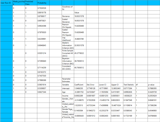
Output
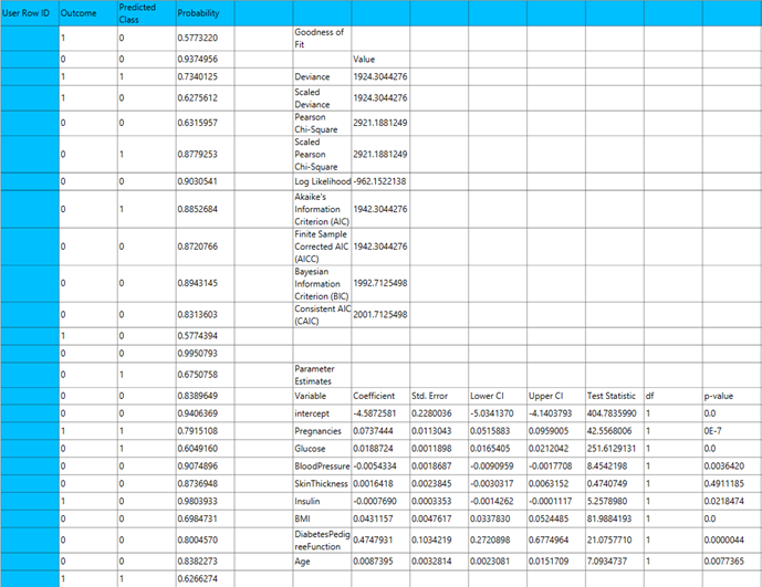
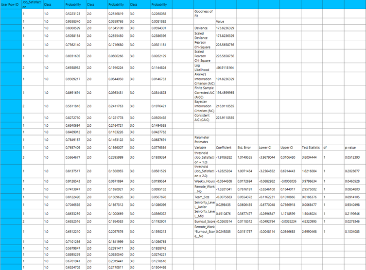
The output of the binary logistic clasification procedure is organized into three main sections: the Predicted Values Table, the Goodness of Fit Statistics, and the Parameter Estimates Table.
- The Predicted Values Table contains the actual values of the dependent variable and the corresponding predicted values generated by the model for each observation.
- The Goodness of Fit Table includes statistical measures that assess how well the model fits the data, such as Deviance, Log-Likelihood, AIC, BIC, and related metrics.
- The Parameter Estimates Table displays the estimated coefficients for each variable in the model, along with standard errors, confidence intervals, test statistics, degrees of freedom, and p-values.
Example
Input
The input datasheet must include one binary dependent variable, which will serve as the target, and at least one column with a continuous or categorical independent variable.
Configuration
- Select
Analytics\(\rightarrow\)Classification\(\rightarrow\)Statistical fitting\(\rightarrow\)Generalized Linear Models - Set the
Type[1] of classification to Binary Logistic. - Specify the
Confidence Level (%)[2] for the test. - Specify
Max Iterations[3]. - Specify the
Maximum Step-Halving[4]. - Select the
Dependent Variable[5]. - Select the
Reference Category[6]. - Select the
Parameter Estimation Method[7]. - Specify the
Maximum Scoring Iterationsif Hybrid option is selected as theParameter Estimation Method[8]. - Specify the
Minimum Change in Parameter Estimates[9]. - Select the
Scale Parameter Method[10]. - Specify the
Value[11] of the scale parameter method if the Fixed value option was chosen as the scale parameter method. - Select the columns by clicking on the arrow buttons [15] and moving columns between the
Excluded Columns[12] andFactors[13] andCovariates[14] lists. Specify Reference Levels[16] for the categorical factors.- Select the prefered
Formula Type[17]. Specify Custom Model Formula[18] for the analysis ifCustomoption is selected. How to specify a custom model formula?- Click on the
Executebutton [19] to perform the Binary Logistic Classification method.
Output
The predictions, Goodness of Fit table and Parameter Estimates table are shown in the output spreadsheet.
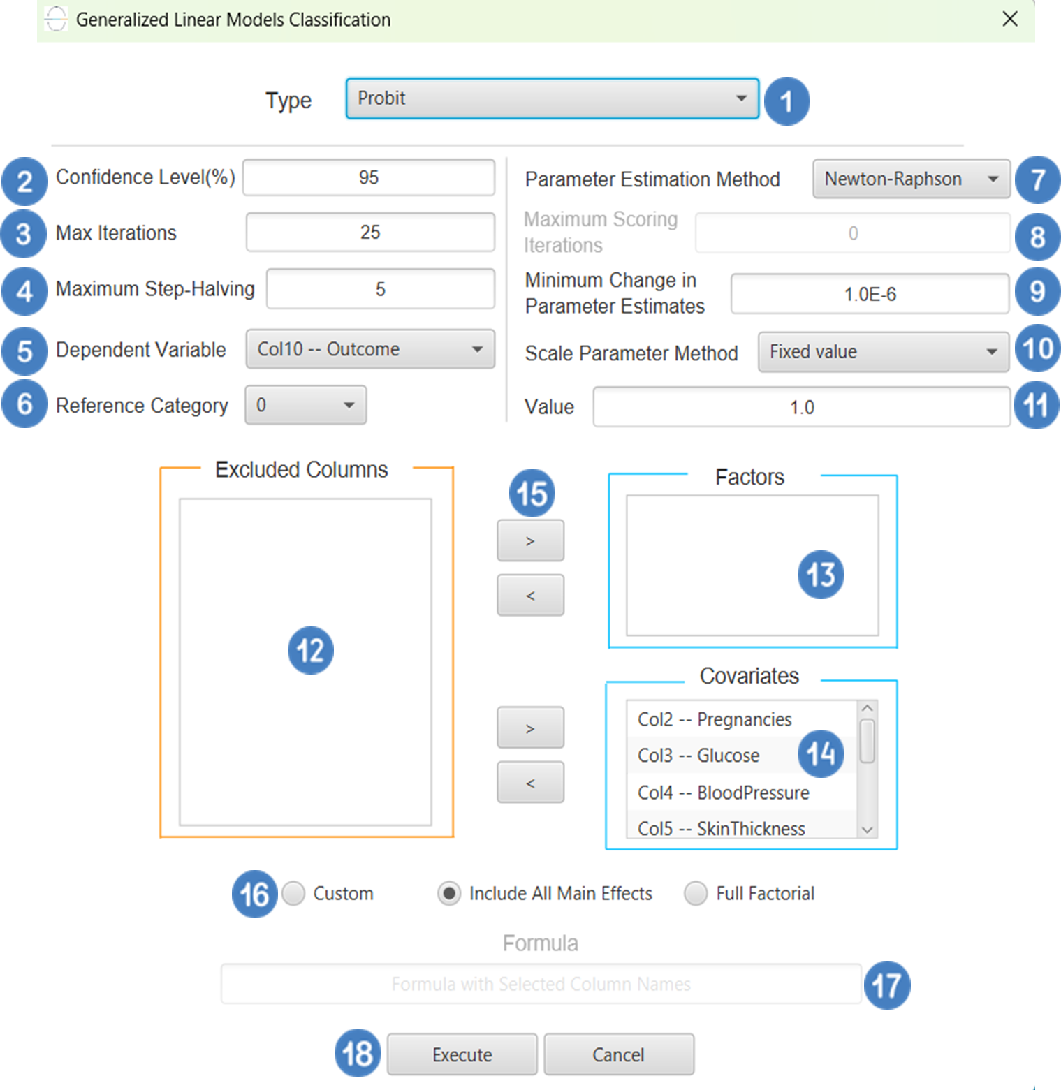
Probit
Probit classification is a type of generalized linear model (GLM) used for modeling a binary outcome variable, like logistic regression. The key difference lies in the link function: while logistic classification uses the logit link, probit classification uses the probit link, which is the inverse of the standard normal cumulative distribution function (CDF). Mathematically, this is expressed as:
Where \(\Phi^{-1}\) is the probit link, and \(\mu\) is the probability of success. The underlying assumption is that there exists a latent (unobserved) continuous variable that follows a standard normal distribution, and the observed binary response is a result of whether this latent variable crosses a certain threshold. Probit classification is often used when the assumption of a normal distribution for the underlying latent variable is justified or preferred, or when the differences in tail behavior between the logistic and normal distributions are relevant.
Use the Probit Classification method by browsing in the top ribbon:
| Analytics \(\rightarrow\) Classification \(\rightarrow\) Statistical fitting \(\rightarrow\) Generalized Linear Models |
And then choosing “Probit” as the Type.
Input
All variables must be specified in the datasheet. Numerical values are required for covariates, while factors may be either textual or numerical. The dependent variable must be binary, consisting of exactly two distinct categories, which can be coded as 0 and 1 or as two unique labels. The design for Probit classification requires at least two columns in the input sheet: one column for the binary dependent variable and at least one column for an independent variable (either a categorical factor or a numerical covariate). Each row corresponds to a single observation.
Configuration
| Confidence Level (%) | Specify the confidence level of the analysis. Values should range from 0 to 100 and correspond to percentages. |
| Max Iterations | Defines the maximum number of iterations the model is allowed to perform during the estimation process. If the model fails to converge before reaching this number, the algorithm stops and returns the values of the last iteration. |
| Maximum Step-Halving | Controls how many times the algorithm is allowed to halve the step size during parameter updates when an iteration leads to worse model fit. |
| Dependent Variable | Select the column that corresponds to values of the dependent variable. |
| Reference Category | Specifies which category of the dependent variable should be used as the reference level when calculating parameter estimates. |
| Parameter Estimation | This option lets you choose how the model parameters will be estimated, Newton-Raphson, Fisher Scoring or Hybrid. |
| Maximum Scoring Iterations | The “Maximum Scoring Iterations” parameter is used when the hybrid estimation method is selected, instead of Newton-Raphson or Fisher scoring alone, and specifies the maximum number of iterations to be performed during the scoring phase. |
| Minimum Change in Parameter Estimates | Sets the tolerance level for convergence — the smallest change in parameter estimates between iterations required to continue optimization. If the change in all parameters is below this value, the algorithm assumes convergence has been reached. |
| Scale Parameter Method | Determines how the scale (error variance) parameter is estimated. Options include: Fixed value, Deviance, or Pearson Chi-square. |
| Value | Specifies the scale parameter value manually, only when Fixed value is selected in the Scale Parameter Method. |
| Factors/Covariates/Excluded Columns | Select manually the columns that correspond to factors and the columns that correspond to covariates through the dialog window: Use the buttons to move columns between the Factors and Covariates list and Excluded Columns list. Single-arrow buttons will move all selected columns and double-arrow buttons will move all columns. At least one covariate or factor column should be specified. |
| Specify Reference Levels | Specify the reference level for each of the categorical factors specified. The default option for each factor is its last level. |
| Formula Type | These options refer to the terms that will be included in the model. The Custom option allows the user to input a formula defining the exact terms to be included. The Main Effects option allows the analysis of a model that only includes all main effects and finally, the Full Factorial option includes both all main effects and all possible interaction terms to build a full model. |
| Specify Custom Model Formula | Specify the model formula used for the analysis if the Custom option is selected. The formula is created in the Custom Formula Creation dialog window by selecting factors and covariates and adding interaction terms up to the required order. Main effects of the included columns are always part of the model and cannot be excluded. |
Output
The output of the Probit classification procedure is organized into three main sections: the Predicted Values Table, the Goodness of Fit Statistics, and the Parameter Estimates Table.
- The Predicted Values Table contains the actual values of the dependent variable and the corresponding predicted values generated by the model for each observation.
- The Goodness of Fit Table includes statistical measures that assess how well the model fits the data, such as Deviance, Log-Likelihood, AIC, BIC, and related metrics.
- The Parameter Estimates Table displays the estimated coefficients for each variable in the model, along with standard errors, confidence intervals, test statistics, degrees of freedom, and p-values.
Example
Input
The input datasheet must include one binary dependent variable, which will serve as the target, and at least one column with a continuous or categorical independent variable.
Configuration
- Select
Analytics\(\rightarrow\)Classification\(\rightarrow\)Statistical fitting\(\rightarrow\)Generalized Linear Models - Set the
Type[1] of classification to Probit. - Specify the
Confidence Level (%)[2] for the test. - Specify
Max Iterations[3]. - Specify the
Maximum Step-Halving[4]. - Select the
Dependent Variable[5]. - Select the
Reference Category[6]. - Select the
Parameter Estimation Method[7]. - Specify the
Maximum Scoring Iterationsif Hybrid option is selected as theParameter Estimation Method[8]. - Specify the
Minimum Change in Parameter Estimates[9]. - Select the
Scale Parameter Method[10]. - Specify the
Value[11] of the scale parameter method if the Fixed value option was chosen as the scale parameter method. - Select the columns by clicking on the arrow buttons [15] and moving columns between the
Excluded Columns[12] andFactors[13] andCovariates[14] lists. Specify Reference Levels[16] for the categorical factors.- Select the prefered
Formula Type[17]. Specify Custom Model Formula[18] for the analysis ifCustomoption is selected. How to specify a custom model formula?- Click on the
Executebutton [19] to perform the Probit Classification method.
Output
The predictions, Goodness of Fit table and Parameter Estimates table are shown in the output spreadsheet.
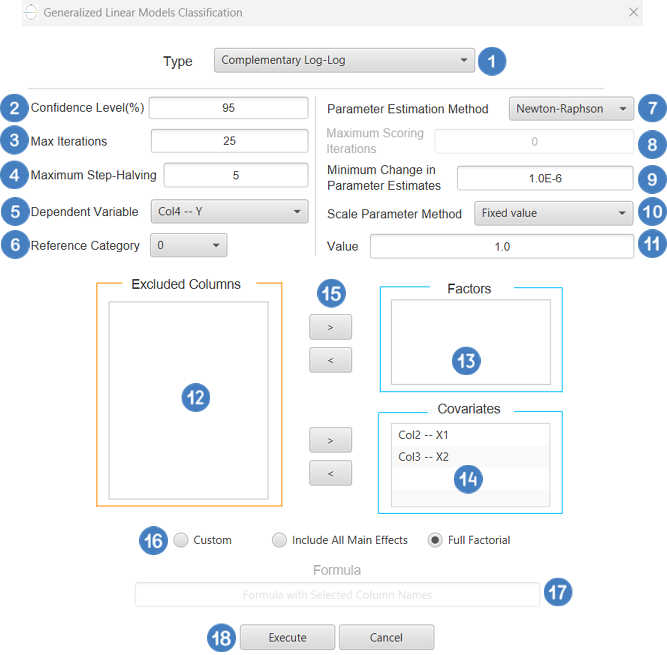
Complementary Log-Log
Complementary log-log classification is a type of generalized linear model (GLM) used for modeling binary outcome data, where the dependent variable consists of two categories (e.g., success/failure, event/no event). Unlike the logit or probit link functions, the cloglog link is defined as:
Where \(\mu\) is the probability of the event occurring. This link function is asymmetric, making it particularly useful when the probability of the event is either very small or very large (i.e., skewed response probabilities). Complementary log-log classification is commonly applied in time-to-event analyses, extreme value modeling, and situations involving hazard functions, such as survival analysis or epidemiological studies, where the event of the interest becomes more likely over time or under certain conditions.
Use the Complementary Log-Log Classification method by browsing in the top ribbon:
| Analytics \(\rightarrow\) Classification \(\rightarrow\) Statistical fitting \(\rightarrow\) Generalized Linear Models |
And then choosing “Complementary Log-Log” as the Type.
Input
All variables must be specified in the datasheet. The dependent variable must be a binary categorical variable, containing exactly two distinct outcomes (e.g., 0 and 1, or two unique labels). The dependent variable should not contain missing entries or values outside the two defined categories. Independent variables may be either numerical or categorical. Categorical variables can be represented using either text labels or numerical codes. The input datasheet must include at least two columns: one for the dependent variable and one or more for the independent variables. Each row should represent a single observation. This model is particularly useful when the probability of the event is highly skewed (close to 0 or 1) and is often applied in contexts involving time-to-event outcomes or hazard-based modeling.
Configuration
| Confidence Level (%) | Specify the confidence level of the analysis. Values should range from 0 to 100 and correspond to percentages. |
| Max Iterations | Defines the maximum number of iterations the model is allowed to perform during the estimation process. If the model fails to converge before reaching this number, the algorithm stops and returns the values of the last iteration. |
| Maximum Step-Halving | Controls how many times the algorithm is allowed to halve the step size during parameter updates when an iteration leads to worse model fit. |
| Dependent Variable | Select the column that corresponds to values of the dependent variable. |
| Reference Category | Specifies which category of the dependent variable should be used as the reference level when calculating parameter estimates. |
| Parameter Estimation | This option lets you choose how the model parameters will be estimated, Newton-Raphson, Fisher Scoring or Hybrid. |
| Maximum Scoring Iterations | The “Maximum Scoring Iterations” parameter is used when the hybrid estimation method is selected, instead of Newton-Raphson or Fisher scoring alone, and specifies the maximum number of iterations to be performed during the scoring phase. |
| Minimum Change in Parameter Estimates | Sets the tolerance level for convergence — the smallest change in parameter estimates between iterations required to continue optimization. If the change in all parameters is below this value, the algorithm assumes convergence has been reached. |
| Scale Parameter Method | Determines how the scale (error variance) parameter is estimated. Options include: Fixed value, Deviance, or Pearson Chi-square. |
| Value | Specifies the scale parameter value manually, only when Fixed value is selected in the Scale Parameter Method. |
| Factors/Covariates/Excluded Columns | Select manually the columns that correspond to factors and the columns that correspond to covariates through the dialog window: Use the buttons to move columns between the Factors and Covariates list and Excluded Columns list. Single-arrow buttons will move all selected columns and double-arrow buttons will move all columns. At least one covariate or factor column should be specified. |
| Specify Reference Levels | Specify the reference level for each of the categorical factors specified. The default option for each factor is its last level. |
| Formula Type | These options refer to the terms that will be included in the model. The Custom option allows the user to input a formula defining the exact terms to be included. The Main Effects option allows the analysis of a model that only includes all main effects and finally, the Full Factorial option includes both all main effects and all possible interaction terms to build a full model. |
| Specify Custom Model Formula | Specify the model formula used for the analysis if the Custom option is selected. The formula is created in the Custom Formula Creation dialog window by selecting factors and covariates and adding interaction terms up to the required order. Main effects of the included columns are always part of the model and cannot be excluded. |
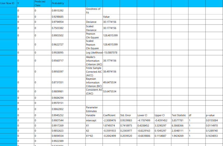
Output
The output of the Complementary Log-Log classification procedure is organized into three main sections: the Predicted Values Table, the Goodness of Fit Statistics, and the Parameter Estimates Table.
- The Predicted Values Table contains the actual values of the dependent variable and the corresponding predicted values generated by the model for each observation.
- The Goodness of Fit Table includes statistical measures that assess how well the model fits the data, such as Deviance, Log-Likelihood, AIC, BIC, and related metrics.
- The Parameter Estimates Table displays the estimated coefficients for each variable in the model, along with standard errors, confidence intervals, test statistics, degrees of freedom, and p-values.
Example
Input
The input datasheet must include one binary dependent variable, which will serve as the target, and at least one column with a continuous or categorical independent variable.
Configuration
- Select
Analytics\(\rightarrow\)Classification\(\rightarrow\)Statistical fitting\(\rightarrow\)Generalized Linear Models - Set the
Type[1] of classification to Complementary Log-Log. - Specify the
Confidence Level (%)[2] for the test. - Specify
Max Iterations[3]. - Specify the
Maximum Step-Halving[4]. - Select the
Dependent Variable[5]. - Select the
Reference Category[6]. - Select the
Parameter Estimation Method[7]. - Specify the
Maximum Scoring Iterationsif Hybrid option is selected as theParameter Estimation Method[8]. - Specify the
Minimum Change in Parameter Estimates[9]. - Select the
Scale Parameter Method[10]. - Specify the
Value[11] of the scale parameter method if the Fixed value option was chosen as the scale parameter method. - Select the columns by clicking on the arrow buttons [15] and moving columns between the
Excluded Columns[12] andFactors[13] andCovariates[14] lists. Specify Reference Levels[16] for the categorical factors.- Select the prefered
Formula Type[17]. Specify Custom Model Formula[18] for the analysis ifCustomoption is selected. How to specify a custom model formula?- Click on the
Executebutton [19] to perform the Complementary Log-Log Classification method.
Output
The predictions, Goodness of Fit table and Parameter Estimates table are shown in the output spreadsheet.
Ordinal Logistic
Ordinal Logistic Classification is a type of generalized linear model (GLM) used when the dependent variable is ordinal-that is, it consists of categories with a natural order but unknown or unequal spacing (e.g., “low”, “medium”, “high”). The most common model used is the proportional odds model, which assumes that the relationship between the predictors and the cumulative probabilities of being at or below a given category is the same across all categories. The typical link function used is the logit link, applied to the cumulative probabilities, resulting in a model of the form:
Where j indexes the thresholds between categories. Ordinal logistic Classification is widely used in fields such as social sciences, medicine, and market research, especially when modeling outcomes like satisfaction ratings, disease severity, or agreement levels.
Use the Ordinal Logistic Classification method by browsing in the top ribbon:
| Analytics \(\rightarrow\) Classification \(\rightarrow\) Statistical fitting \(\rightarrow\) Generalized Linear Models |
And then choosing “Ordinal Logistic” as the Type.
Input
All variables must be specified in the datasheet. The dependent variable must be ordinal and expressed using numerical codes only (e.g., 1, 2, 3), where higher values represent higher levels in the ordering. It should consist of three or more ordered categories and must not contain any missing values or codes outside the defined ordinal range. For logical and interpretable results, the values in the dependent variable column should reflect the correct ordinal ranking for each observation. Independent variables may be either numerical or categorical. Categorical predictors can be represented using either text labels or numerical codes, but each entry should clearly correspond to the level of the factor it represents. The input datasheet must include at least two columns: one for the numerically coded ordinal dependent variable, and one or more for the independent variables. Each row must represent a single observation. This model is particularly suited for estimating the likelihood of an observation falling into a higher or lower category along an ordered scale.
Configuration
| Confidence Level (%) | Specify the confidence level of the analysis. Values should range from 0 to 100 and correspond to percentages. |
| Max Iterations | Defines the maximum number of iterations the model is allowed to perform during the estimation process. If the model fails to converge before reaching this number, the algorithm stops and returns the values of the last iteration. |
| Maximum Step-Halving | Controls how many times the algorithm is allowed to halve the step size during parameter updates when an iteration leads to worse model fit. |
| Dependent Variable | Select the column that corresponds to values of the dependent variable. |
| Parameter Estimation | This option lets you choose how the model parameters will be estimated, Newton-Raphson, Fisher Scoring or Hybrid. |
| Maximum Scoring Iterations | The “Maximum Scoring Iterations” parameter is used when the hybrid estimation method is selected, instead of Newton-Raphson or Fisher scoring alone, and specifies the maximum number of iterations to be performed during the scoring phase. |
| Minimum Change in Parameter Estimates | Sets the tolerance level for convergence — the smallest change in parameter estimates between iterations required to continue optimization. If the change in all parameters is below this value, the algorithm assumes convergence has been reached. |
| Scale Parameter Method | Determines how the scale (error variance) parameter is estimated. Options include: Fixed value, Deviance, or Pearson Chi-square. |
| Value | Specifies the scale parameter value manually, only when Fixed value is selected in the Scale Parameter Method. |
| Factors/Covariates/Excluded Columns | Select manually the columns that correspond to factors and the columns that correspond to covariates through the dialog window: Use the buttons to move columns between the Factors and Covariates list and Excluded Columns list. Single-arrow buttons will move all selected columns and double-arrow buttons will move all columns. At least one covariate or factor column should be specified. |
| Specify Reference Levels | Specify the reference level for each of the categorical factors specified. The default option for each factor is its last level. |
| Formula Type | These options refer to the terms that will be included in the model. The Custom option allows the user to input a formula defining the exact terms to be included. The Main Effects option allows the analysis of a model that only includes all main effects and finally, the Full Factorial option includes both all main effects and all possible interaction terms to build a full model. |
| Specify Custom Model Formula | Specify the model formula used for the analysis if the Custom option is selected. The formula is created in the Custom Formula Creation dialog window by selecting factors and covariates and adding interaction terms up to the required order. Main effects of the included columns are always part of the model and cannot be excluded. |
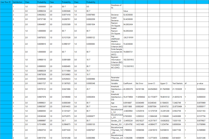
Output
The output of the ordinal logistic Classification procedure is organized into three main sections: the Predicted Probabilities Table, the Goodness of Fit Statistics, and the Parameter Estimates Table.
- The Predicted Probabilities Table displays the actual observed values of the ordinal dependent variable in the first column, followed by the predicted probabilities of each observation belonging to each outcome category. These probabilities are based on the fitted model and indicate how likely each case is to fall into each level of the ordinal outcome.
- The Goodness of Fit Table includes statistical measures that assess how well the model fits the data, such as Deviance, Log-Likelihood, AIC, BIC, and related metrics.
- The Parameter Estimates Table displays the estimated coefficients for the model. The first rows refer to the thresholds (cut-points) between the ordinal categories of the dependent variable. These are followed by the coefficients for the independent variables, showing their effect on the likelihood of being in a higher category. The table also includes the standard errors, 95% confidence intervals, test statistics, degrees of freedom, and p-values used to assess the statistical significance of each term in the model.
Example
Input
The input datasheet must include one target variable with ordered categories, and at least one continuous or categorical independent variable.

Configuration
- Select
Analytics\(\rightarrow\)Classification\(\rightarrow\)Statistical fitting\(\rightarrow\)Generalized Linear Models - Set the
Type[1] of classification to Ordinal Logistic. - Specify the
Confidence Level (%)[2] for the test. - Specify
Max Iterations[3]. - Specify the
Maximum Step-Halving[4]. - Select the
Dependent Variable[5]. - Select the
Parameter Estimation Method[6]. - Specify the
Maximum Scoring Iterationsif Hybrid option is selected as theParameter Estimation Method[7]. - Specify the
Minimum Change in Parameter Estimates[8]. - Select the
Scale Parameter Method[9]. - Specify the
Value[10] of the scale parameter method if the Fixed value option was chosen as the scale parameter method. - Select the columns by clicking on the arrow buttons [14] and moving columns between the
Excluded Columns[11] andFactors[12] andCovariates[13] lists. Specify Reference Levels[15] for the categorical factors.- Select the prefered
Formula Type[16]. Specify Custom Model Formula[17] for the analysis ifCustomoption is selected. How to specify a custom model formula?- Click on the
Executebutton [18] to perform the Ordinal Logistic Classification method.
Output
The predictions, Goodness of Fit table and Parameter Estimates table are shown in the output spreadsheet.
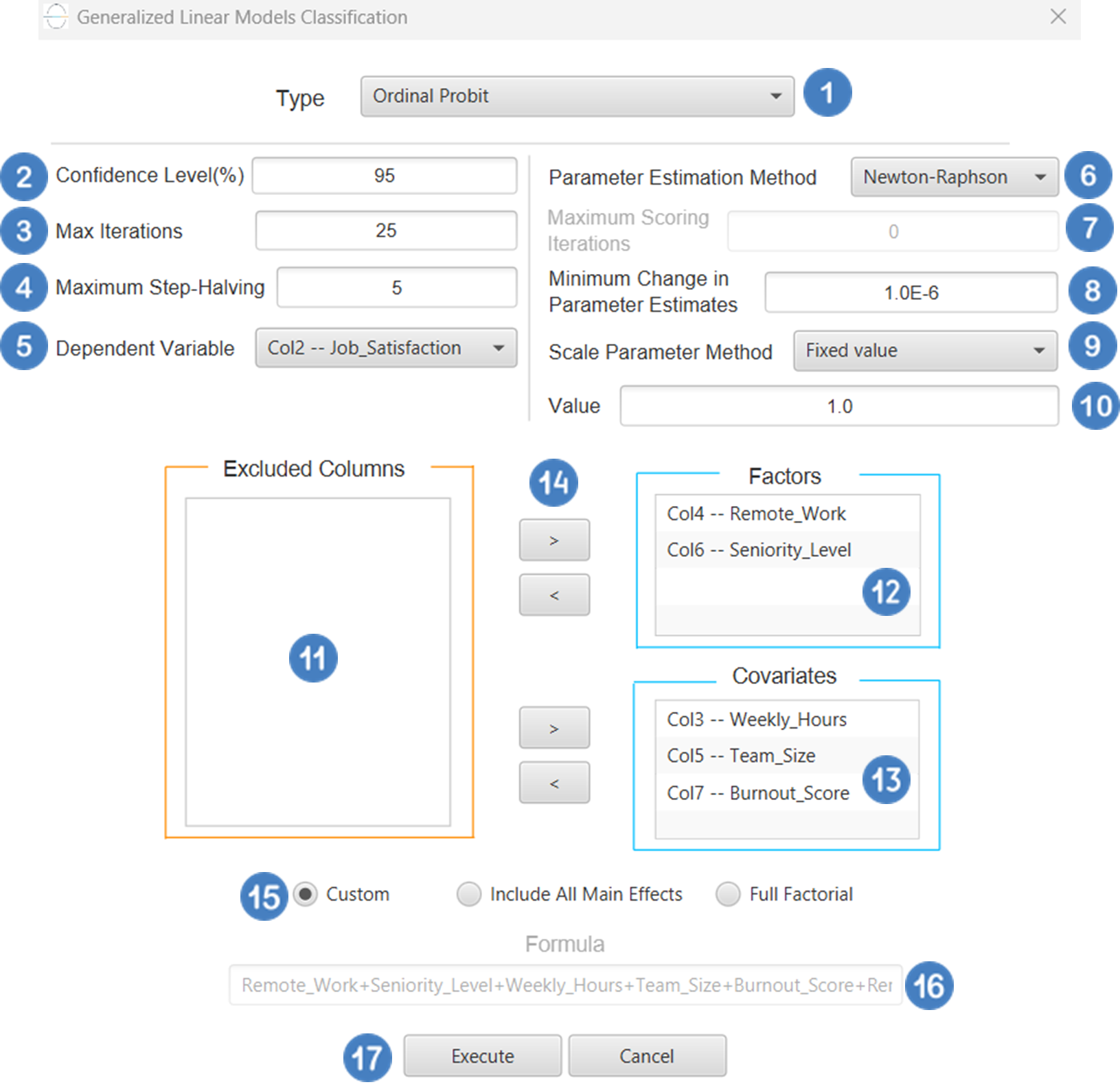
Ordinal Probit
Ordinal Classification, as discussed earlier, is a type of generalized linear model (GLM) used when the dependent variable is ordinal—that is, it consists of categories with a natural order but unknown or unequal spacing (e.g., “low”, “medium”, “high”). A common variant of this model uses the probit link function, which, instead of the logistic function, applies to the standard normal cumulative distribution function (CDF) to model the cumulative probabilities. The model takes the following form:
Where j indexes the thresholds between categories, xβ represents the linear predictor, and the probit function is the inverse of the standard normal CDF (\(\Phi^{-1}\)). The interpretation is broadly like that of the proportional odds model with the logit link, although the probit model assumes that the underlying latent errors follow a standard normal distribution, as opposed to the logistic distribution assumed in the logit case. The probit link is commonly used in fields such as psychometrics and economics, where the assumption of normally distributed errors may be more appropriate. It is also useful when comparing different GLM approaches or when theoretical considerations favor the normal distribution over the logistic.
Use the Ordinal Probit Classification method by browsing in the top ribbon:
| Analytics \(\rightarrow\) Classification \(\rightarrow\) Statistical fitting \(\rightarrow\) Generalized Linear Models |
And then choosing “Ordinal Probit” as the Type.
Input
All variables must be specified in the datasheet. The dependent variable must be ordinal and expressed using numerical codes only (e.g., 1, 2, 3), where higher values represent higher levels in the ordering. It should consist of three or more ordered categories and must not contain any missing values or codes outside the defined ordinal range. For logical and interpretable results, the values in the dependent variable column should reflect the correct ordinal ranking for each observation. Independent variables may be either numerical or categorical. Categorical predictors can be represented using either text labels or numerical codes, but each entry should clearly correspond to the level of the factor it represents. The input datasheet must include at least two columns: one for the numerically coded ordinal dependent variable, and one or more for the independent variables. Each row must represent a single observation. This model is particularly suited for estimating the likelihood of an observation falling into a higher or lower category along an ordered scale.
Configuration
| Confidence Level (%) | Specify the confidence level of the analysis. Values should range from 0 to 100 and correspond to percentages. |
| Max Iterations | Defines the maximum number of iterations the model is allowed to perform during the estimation process. If the model fails to converge before reaching this number, the algorithm stops and returns the values of the last iteration. |
| Maximum Step-Halving | Controls how many times the algorithm is allowed to halve the step size during parameter updates when an iteration leads to worse model fit. |
| Dependent Variable | Select the column that corresponds to values of the dependent variable. |
| Parameter Estimation | This option lets you choose how the model parameters will be estimated, Newton-Raphson, Fisher Scoring or Hybrid. |
| Maximum Scoring Iterations | The “Maximum Scoring Iterations” parameter is used when the hybrid estimation method is selected, instead of Newton-Raphson or Fisher scoring alone, and specifies the maximum number of iterations to be performed during the scoring phase. |
| Minimum Change in Parameter Estimates | Sets the tolerance level for convergence — the smallest change in parameter estimates between iterations required to continue optimization. If the change in all parameters is below this value, the algorithm assumes convergence has been reached. |
| Scale Parameter Method | Determines how the scale (error variance) parameter is estimated. Options include: Fixed value, Deviance, or Pearson Chi-square. |
| Value | Specifies the scale parameter value manually, only when Fixed value is selected in the Scale Parameter Method. |
| Factors/Covariates/Excluded Columns | Select manually the columns that correspond to factors and the columns that correspond to covariates through the dialog window: Use the buttons to move columns between the Factors and Covariates list and Excluded Columns list. Single-arrow buttons will move all selected columns and double-arrow buttons will move all columns. At least one covariate or factor column should be specified. |
| Specify Reference Levels | Specify the reference level for each of the categorical factors specified. The default option for each factor is its last level. |
| Formula Type | These options refer to the terms that will be included in the model. The Custom option allows the user to input a formula defining the exact terms to be included. The Main Effects option allows the analysis of a model that only includes all main effects and finally, the Full Factorial option includes both all main effects and all possible interaction terms to build a full model. |
| Specify Custom Model Formula | Specify the model formula used for the analysis if the Custom option is selected. The formula is created in the Custom Formula Creation dialog window by selecting factors and covariates and adding interaction terms up to the required order. Main effects of the included columns are always part of the model and cannot be excluded. |
Output
The output of the ordinal probit classification procedure is organized into three main sections: the Predicted Probabilities Table, the Goodness of Fit Statistics, and the Parameter Estimates Table.
- The Predicted Probabilities Table displays the actual observed values of the ordinal dependent variable in the first column, followed by the predicted probabilities of each observation belonging to each outcome category. These probabilities are based on the fitted model and indicate how likely each case is to fall into each level of the ordinal outcome.
- The Goodness of Fit Table includes statistical measures that assess how well the model fits the data, such as Deviance, Log-Likelihood, AIC, BIC, and related metrics.
- The Parameter Estimates Table displays the estimated coefficients for the model. The first rows refer to the thresholds (cut-points) between the ordinal categories of the dependent variable. These are followed by the coefficients for the independent variables, showing their effect on the likelihood of being in a higher category. The table also includes the standard errors, 95% confidence intervals, test statistics, degrees of freedom, and p-values used to assess the statistical significance of each term in the model.
Example
Input
The input datasheet must include one target variable with ordered categories, and at least one continuous or categorical independent variable.
Configuration
- Select
Analytics\(\rightarrow\)Classification\(\rightarrow\)Statistical fitting\(\rightarrow\)Generalized Linear Models - Set the
Type[1] of classification to Ordinal Probit. - Specify the
Confidence Level (%)[2] for the test. - Specify
Max Iterations[3]. - Specify the
Maximum Step-Halving[4]. - Select the
Dependent Variable[5]. - Select the
Parameter Estimation Method[6]. - Specify the
Maximum Scoring Iterationsif Hybrid option is selected as theParameter Estimation Method[7]. - Specify the
Minimum Change in Parameter Estimates[8]. - Select the
Scale Parameter Method[9]. - Specify the
Value[10] of the scale parameter method if the Fixed value option was chosen as the scale parameter method. - Select the columns by clicking on the arrow buttons [14] and moving columns between the
Excluded Columns[11] andFactors[12] andCovariates[13] lists. Specify Reference Levels[15] for the categorical factors.- Select the prefered
Formula Type[16]. Specify Custom Model Formula[17] for the analysis ifCustomoption is selected. How to specify a custom model formula?- Click on the
Executebutton [18] to perform the Ordinal Probit Classification method.
Output
The predictions, Goodness of Fit table and Parameter Estimates table are shown in the output spreadsheet.
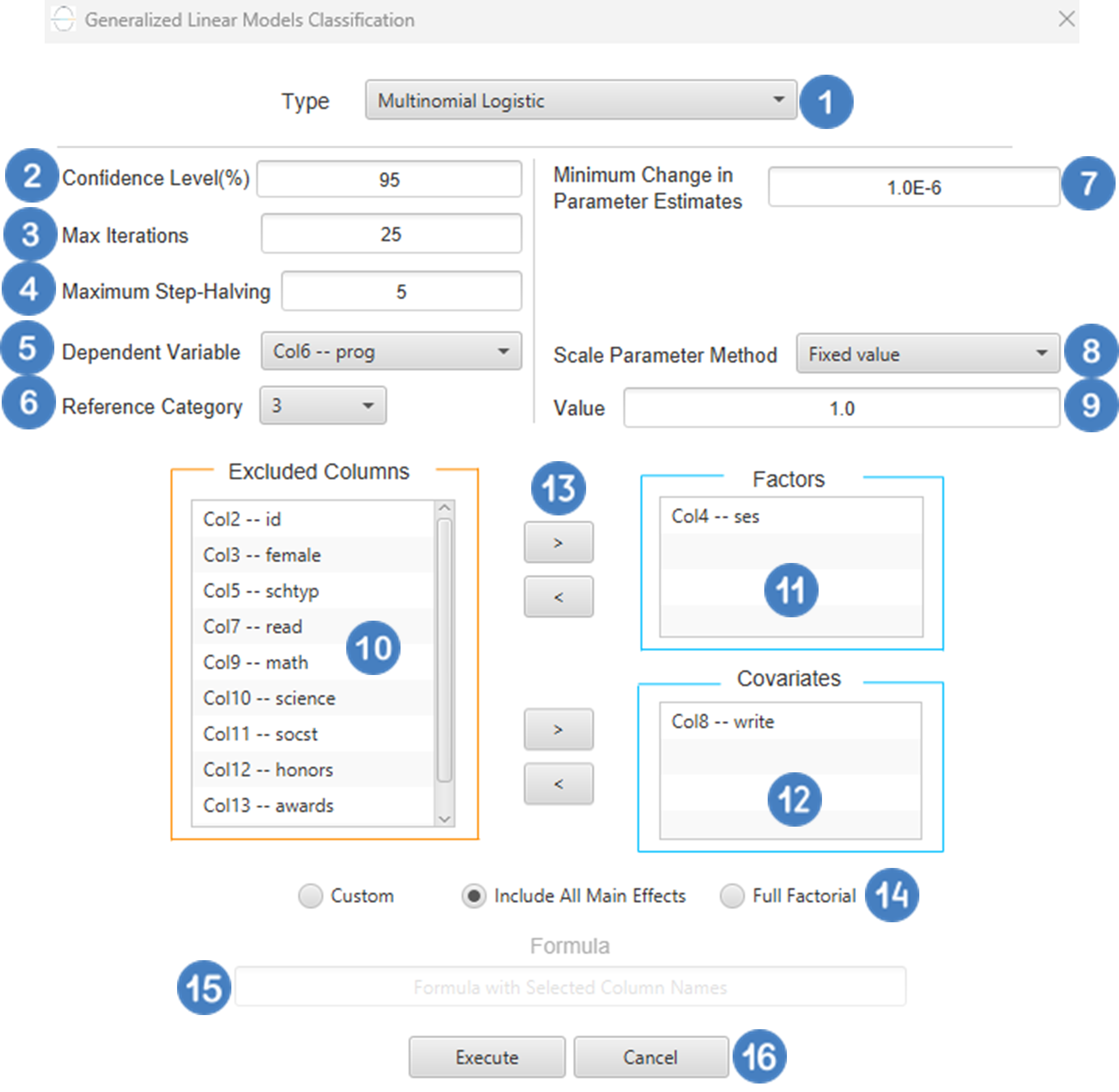
Multinomial Logistic
Multinomial Logistic Classification is a classification method that generalizes logistic classification to multiclass problems, i.e. with more than two possible discrete outcomes that cannot be ordered. This type of GLM assumes the response variable follows a multinomial distribution which is a generalization of the binomial distribution for more than two categories. The link function used is the SoftMax function which for a response variable Y with K possible classes is defined as:
Use the Multinomial Logistic Classification method by browsing in the top ribbon:
| Analytics \(\rightarrow\) Classification \(\rightarrow\) Statistical fitting \(\rightarrow\) Generalized Linear Models |
And then choosing “Multinomial Logistic” as the Type.
Input
All variables must be specified in the datasheet. The dependent variable must be categorical with more than two distinct values that do not follow any inherent or numerical order (e.g., categories such as “red”, “yellow”, “blue”). The dependent variable should not contain missing values or categories outside the defined set. Independent variables may be either numerical or categorical. Categorical variables can be represented using either text labels or numerical codes. The input datasheet must include at least two columns: one for the dependent variable and one or more for the independent variables. Each row should represent a single observation. This model is appropriate when the outcome involves nominal categories with no meaningful order and is typically used in multi-class classification problems.
Configuration
| Confidence Level (%) | Specify the confidence level of the analysis. Values should range from 0 to 100 and correspond to percentages. |
| Max Iterations | Defines the maximum number of iterations the model is allowed to perform during the estimation process. If the model fails to converge before reaching this number, the algorithm stops and returns the values of the last iteration. |
| Maximum Step-Halving | Controls how many times the algorithm is allowed to halve the step size during parameter updates when an iteration leads to worse model fit. |
| Dependent Variable | Select the column that corresponds to values of the dependent variable. |
| Reference Category | Specifies which category of the dependent variable should be used as the reference level when calculating parameter estimates. |
| Minimum Change in Parameter Estimates | Sets the tolerance level for convergence — the smallest change in parameter estimates between iterations required to continue optimization. If the change in all parameters is below this value, the algorithm assumes convergence has been reached. |
| Scale Parameter Method | Determines how the scale (error variance) parameter is estimated. Options include: Fixed value, Deviance, or Pearson Chi-square. |
| Value | Specifies the scale parameter value manually, only when Fixed value is selected in the Scale Parameter Method. |
| Factors/Covariates/Excluded Columns | Select manually the columns that correspond to factors and the columns that correspond to covariates through the dialog window: Use the buttons to move columns between the Factors and Covariates list and Excluded Columns list. Single-arrow buttons will move all selected columns and double-arrow buttons will move all columns. At least one covariate or factor column should be specified. |
| Specify Reference Levels | Specify the reference level for each of the categorical factors specified. The default option for each factor is its last level. |
| Formula Type | These options refer to the terms that will be included in the model. The Custom option allows the user to input a formula defining the exact terms to be included. The Main Effects option allows the analysis of a model that only includes all main effects and finally, the Full Factorial option includes both all main effects and all possible interaction terms to build a full model. |
| Specify Custom Model Formula | Specify the model formula used for the analysis if the Custom option is selected. The formula is created in the Custom Formula Creation dialog window by selecting factors and covariates and adding interaction terms up to the required order. Main effects of the included columns are always part of the model and cannot be excluded. |
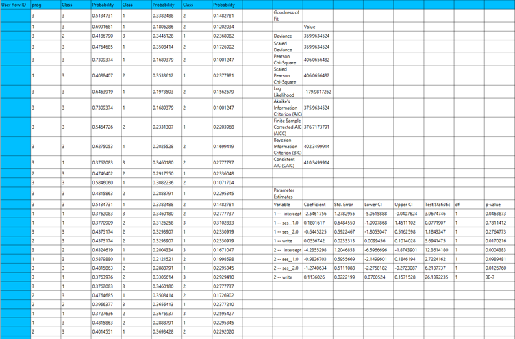
Output
The output of the multinomial logistic classification procedure is organized into three main sections: the Predicted Probabilities Table, the Goodness of Fit Statistics, and the Parameter Estimates Table.
- The Predicted Probabilities Table lists, for each observation, the predicted probability of belonging to each possible outcome category, along with the corresponding category label.Each row represents the model’s estimated probability that a specific case falls into a given outcome category, based on the fitted multinomial logistic classification model.
- The Goodness of Fit Table includes statistical measures that assess how well the model fits the data, such as Deviance, Log-Likelihood, AIC, BIC, and related metrics.
- The Parameter Estimates Table displays the estimated coefficients for the model. The first rows refer to the thresholds (cut-points) between the ordinal categories of the dependent variable. These are followed by the coefficients for the independent variables, showing their effect on the likelihood of being in a higher category. The table also includes the standard errors, 95% confidence intervals, test statistics, degrees of freedom, and p-values used to assess the statistical significance of each term in the model.
Example
Input
The input datasheet must include one nominal dependent variable with three or more unordered categories, which will serve as the target, and at least one column containing a continuous or categorical independent variable.
Configuration
- Select
Analytics\(\rightarrow\)Classification\(\rightarrow\)Statistical fitting\(\rightarrow\)Generalized Linear Models - Set the
Type[1] of classification to Multinomial Logistic. - Specify the
Confidence Level (%)[2] for the test. - Specify
Max Iterations[3]. - Specify the
Maximum Step-Halving[4]. - Select the
Dependent Variable[5]. - Select the
Reference Category[6]. - Specify the
Minimum Change in Parameter Estimates[7]. - Select the
Scale Parameter Method[8]. - Specify the
Value[9] of the scale parameter method if the Fixed value option was chosen as the scale parameter method. - Select the columns by clicking on the arrow buttons [13] and moving columns between the
Excluded Columns[10] andFactors[11] andCovariates[12] lists. Specify Reference Levels[14] for the categorical factors.- Select the prefered
Formula Type[15]. Specify Custom Model Formula[16] for the analysis ifCustomoption is selected. How to specify a custom model formula?- Click on the
Executebutton [17] to perform the Multinomial Logistic Classification method.
Output
The predictions, Goodness of Fit table and Parameter Estimates table are shown in the output spreadsheet.
Generalized Estimating Equations
Generalized Estimating Equations (GEEs) extend Generalized Linear Models (GLMs) to handle correlated or clustered response data, such as repeated measures or longitudinal observations. GEEs are particularly useful when responses are not independent, as they allow for within-subject correlation, making them ideal for analyzing data collected over time or across related units. A GEE model consists of the following key components:
- Mean Structure: Like GLMs, the expected value of the response variable is modeled using a linear predictor :
Where \(x_i\) is the vector of predictors and \(\beta\) is the vector of coefficients.
- Link Function: A monotonic function \(g(∙)\) that links the mean of the response \(\mu_i= E[y_i]\) to the linear predictor, so that \(g(\mu_i)=\eta_i\).
- Working Correlation Matrix: Specifies the assumed correlation structure among repeated observations within the same subject. Common structures include:
- Independent: assumes no within-subject correlation.
- Exchangeable: assumes equal correlation between all pairs of observations.
- AR(1): assumes correlations decrease with time distance.
- Unstructured: allows a distinct correlation for each pair of observations, with no constraints.
- M-dependent: assumes nonzero correlations only up to lag M, and zero correlations beyond that distance.
GEE estimation relies on solving quasi-likelihood equations rather than maximizing a full likelihood function, making it a semi-parametric approach. Parameters are estimated using iterative methods such as iteratively reweighted least squares (IRLS), and standard errors are typically computed using robust estimators to ensure valid inference even if the correlation structure is misspecified. In GEE models, a subject variable is required to identify the unit over which repeated measurements occur (e.g., patient ID). Optionally, a within-subject variable (e.g., time or visit number) can be specified to define the ordering of repeated measurements. Cases are usually sorted by subject and within-subject variables to ensure correct modeling of correlation patterns. The robust covariance estimator is the default choice, providing consistent standard errors under mild assumptions. The model-based estimator may be more efficient if the correlation structure is correctly specified, but it is more sensitive to misspecification. Categorical variables are encoded using dummy coding, as in GLMs. The reference category is omitted by default to avoid multicollinearity and serve as a baseline for interpreting effects.
Each variant of this method is specified by the distribution of the response variable and the link function used. In the table below we specify the distribution and link function used for each variant:
| GEE Variant | Distribution | Link Function |
| Binary Logistic | Binomial | Logit |
| Probit | Binomial | Probit |
| Complementary Log-Log | Binomial | CLogLog |
| Ordinal Logistic | Multinomial | Logit |
| Ordinal Probit | Multinomial | Probit |
Binary Logistic
Use the Binary Logistic Classification method by browsing in the top ribbon:
| Analytics \(\rightarrow\) Classification \(\rightarrow\) Statistical fitting \(\rightarrow\) Generalized Estimating Equations |
And then choosing “Binary Logistic” as the Type.
Input
All variables must be specified in the datasheet. The dependent variable must be binary, as Binary Logistic Classification within the GEE framework models dichotomous outcomes. The binary outcome should be coded as 0 and 1. Covariates should be numerical, while categorical predictors (factors) can be represented using either text labels or numeric codes. The input datasheet must include at least two columns: one for the dependent variable and one or more for the independent variables (covariates or factors). Each row should correspond to a single observation. Additionally, a subject identifier column is required to define clusters of repeated measurements, and optionally a within-subject variable (e.g., time) to specify the order of observations within each subject.
Configuration
| Confidence Level (%) | Specify the confidence level of the analysis. Values should range from 0 to 100 and correspond to percentages. |
| Max Iterations | Defines the maximum number of iterations the model is allowed to perform during the estimation process. If the model fails to converge before reaching this number, the algorithm stops and returns the values of the last iteration. |
| Iterations Between Updates | Defines how often the working correlation matrix is updated during estimation. |
| Dependent Variable | Select the column that corresponds to values of the dependent variable. |
| Reference Category | Specifies which category of the dependent variable should be used as the reference level when calculating parameter estimates. |
| Minimum Change in Parameter Estimates | Sets the tolerance level for convergence — the smallest change in parameter estimates between iterations required to continue optimization. If the change in all parameters is below this value, the algorithm assumes convergence has been reached. |
| Hessian Convergence | Specifies a threshold for convergence based on the second derivatives (Hessian matrix). |
| Scale Parameter | Adjusts the variance of the model. |
| Within Subject | Selects the column that defines the ordering of repeated observations within each subject. |
| Structure | Defines the working correlation structure for repeated measurements within subjects. Choices include Independent, Exchangeable, AR(1), Unstructured and M-Dependent. |
| M | In the M-Dependent correlation structure, M specifies the maximum number of consecutive observations within each cluster that are assumed to be correlated, with correlations set to zero for observations more than M time points apart. M must be an integer in the range from 1 to (number of within-subject observations – 1). |
| Covariance Matrix | In the Covariance Matrix option, the user selects how the model’s standard errors will be estimated. The Robust estimator is resistant to misspecification of the correlation structure, while the Model-based estimator assumes the specified correlation is correct. |
| Subjects/Factors/Covariates/Excluded Columns | Select manually the columns that correspond to subjects, factors and the columns that correspond to covariates through the dialog window: Use the buttons to move columns between the Subjects, Factors and Covariates list and Excluded Columns list. Single-arrow buttons will move all selected columns. At least one covariate or factor column should be specified. Also, a column for the Subject is required. |
| Specify Reference Levels | Specify the reference level for each of the categorical factors specified. The default option for each factor is its last level. |
| Formula Type | These options refer to the terms that will be included in the model. The Custom option allows the user to input a formula defining the exact terms to be included. The Main Effects option allows the analysis of a model that only includes all main effects and finally, the Full Factorial option includes both all main effects and all possible interaction terms to build a full model. |
| Specify Custom Model Formula | Specify the model formula used for the analysis if the Custom option is selected. The formula is created in the Custom Formula Creation dialog window by selecting factors and covariates and adding interaction terms up to the required order. Main effects of the included columns are always part of the model and cannot be excluded. |
Output
The output of the Generalized Estimating Equations (GEEs) procedure is organized into three main sections: the Predicted Values Table, the Parameter Estimates Table and the Working Correlation Matrix.
- The Predicted Values Table shows the fitted values for the dependent variable on the specified model.
- The Parameter Estimates Table includes the estimated coefficients for the independent variables. Each row corresponds to a predictor and includes its coefficient, standard error, confidence interval, test statistic, degrees of freedom, and p-value.
- The Working Correlation Matrix displays the estimated correlations between repeated measurements of the same subject over time.
Example
Input
The dataset must include a binary target variable suitable for modeling with binary logistic classification. The binary outcome should be coded as 0 and 1. It should also contain at least one independent variable, which can be continuous or categorical. In addition, the dataset must include a subject identifier to group repeated observations from the same individual or unit, as well as a within-subject time or measurement indicator to reflect the longitudinal or clustered nature of the data.
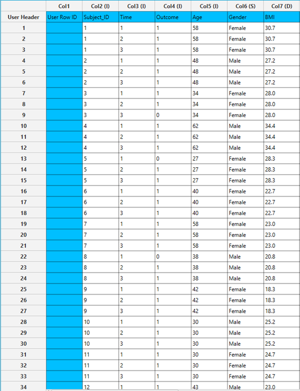
Configuration
- Select
Analytics\(\rightarrow\)Classification\(\rightarrow\)Statistical fitting\(\rightarrow\)Generalized Estimating Equations. - Set the
Type[1] of classification to Binary Logistic. - Specify the
Confidence Level (%)[2] for the test. - Specify
Max Iterations[3]. - Specify
Iterations Between Updates[4]. - Select the
Dependent Variable[5]. - Select the
Reference Category[6]. - Specify the
Minimum Change in Parameter Estimates[7]. - Specify the
Hessian Convergence[8]. - Specify the
Scale Parameter[9]. - Select the
Within Subject[10]. - Select the
working correlation Structureand specify the value ofMif you select M-Dependent as the correlation structure. [11]. - Select the method used to estimate the
covariance matrix[12] of the standard errors. - Select the columns by clicking on the arrow buttons [17] and moving columns between the
Excluded Columns[13] andSubjects[14] andFactors[15] andCovariates[16] lists. Specify Reference Levels[18] for the categorical factors.- Select the prefered
Formula Type[19]. Specify Custom Model Formula[20] for the analysis ifCustomoption is selected. How to specify a custom model formula?- Click on the
Executebutton [21] to perform the Binary Logistic Classification method.
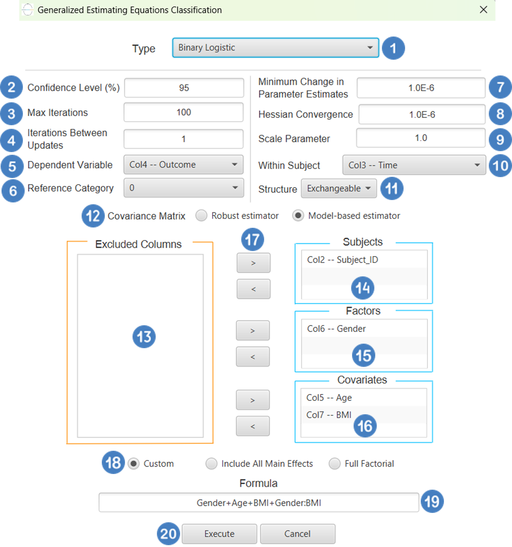
Output
The Predictions, Parameter Estimates table and Working Correlation Matrix are shown in the output spreadsheet.
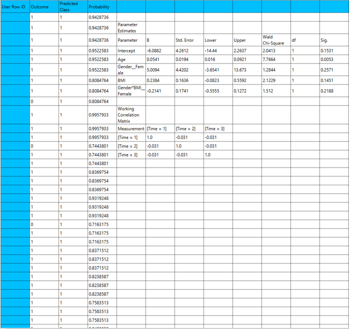
Probit
Use the Probit Classification method by browsing in the top ribbon:
| Analytics \(\rightarrow\) Classification \(\rightarrow\) Statistical fitting \(\rightarrow\) Generalized Estimating Equations |
And then choosing “Probit” as the Type.
Input
All variables must be specified in the datasheet. The dependent variable must be binary, as Probit Classification within the GEE framework models dichotomous outcomes using a cumulative normal (probit) link function. The binary outcome should be coded as 0 and 1. Covariates should be numerical, while categorical predictors (factors) can be represented using either text labels or numeric codes. The input datasheet must include at least two columns: one for the dependent variable and one or more for the independent variables (covariates or factors). Each row should correspond to a single observation. Additionally, a subject identifier column is required to define clusters of repeated measurements, and optionally a within-subject variable (e.g., time) to specify the order of observations within each subject.
Configuration
| Confidence Level (%) | Specify the confidence level of the analysis. Values should range from 0 to 100 and correspond to percentages. |
| Max Iterations | Defines the maximum number of iterations the model is allowed to perform during the estimation process. If the model fails to converge before reaching this number, the algorithm stops and returns the values of the last iteration. |
| Iterations Between Updates | Defines how often the working correlation matrix is updated during estimation. |
| Dependent Variable | Select the column that corresponds to values of the dependent variable. |
| Reference Category | Specifies which category of the dependent variable should be used as the reference level when calculating parameter estimates. |
| Minimum Change in Parameter Estimates | Sets the tolerance level for convergence — the smallest change in parameter estimates between iterations required to continue optimization. If the change in all parameters is below this value, the algorithm assumes convergence has been reached. |
| Hessian Convergence | Specifies a threshold for convergence based on the second derivatives (Hessian matrix). |
| Scale Parameter | Adjusts the variance of the model. |
| Within Subject | Selects the column that defines the ordering of repeated observations within each subject. |
| Structure | Defines the working correlation structure for repeated measurements within subjects. Choices include Independent, Exchangeable, AR(1), Unstructured and M-Dependent. |
| M | In the M-Dependent correlation structure, M specifies the maximum number of consecutive observations within each cluster that are assumed to be correlated, with correlations set to zero for observations more than M time points apart. M must be an integer in the range from 1 to (number of within-subject observations – 1). |
| Covariance Matrix | In the Covariance Matrix option, the user selects how the model’s standard errors will be estimated. The Robust estimator is resistant to misspecification of the correlation structure, while the Model-based estimator assumes the specified correlation is correct. |
| Subjects/Factors/Covariates/Excluded Columns | Select manually the columns that correspond to subjects, factors and the columns that correspond to covariates through the dialog window: Use the buttons to move columns between the Subjects, Factors and Covariates list and Excluded Columns list. Single-arrow buttons will move all selected columns. At least one covariate or factor column should be specified. Also, a column for the Subject is required. |
| Specify Reference Levels | Specify the reference level for each of the categorical factors specified. The default option for each factor is its last level. |
| Formula Type | These options refer to the terms that will be included in the model. The Custom option allows the user to input a formula defining the exact terms to be included. The Main Effects option allows the analysis of a model that only includes all main effects and finally, the Full Factorial option includes both all main effects and all possible interaction terms to build a full model. |
| Specify Custom Model Formula | Specify the model formula used for the analysis if the Custom option is selected. The formula is created in the Custom Formula Creation dialog window by selecting factors and covariates and adding interaction terms up to the required order. Main effects of the included columns are always part of the model and cannot be excluded. |
Output
The output of the Generalized Estimating Equations (GEEs) procedure is organized into three main sections: the Predicted Values Table, the Parameter Estimates Table and the Working Correlation Matrix.
- The Predicted Values Table shows the fitted values for the dependent variable on the specified model.
- The Parameter Estimates Table includes the estimated coefficients for the independent variables. Each row corresponds to a predictor and includes its coefficient, standard error, confidence interval, test statistic, degrees of freedom, and p-value.
- The Working Correlation Matrix displays the estimated correlations between repeated measurements of the same subject over time.
Example
Input
The dataset must include a binary target variable suitable for modeling with binary probit classification. The binary outcome should be coded as 0 and 1. It should also contain at least one independent variable, which can be continuous or categorical. In addition, the dataset must include a subject identifier to group repeated observations from the same individual or unit, as well as a within-subject time or measurement indicator to reflect the longitudinal or clustered nature of the data. The structure of the dataset should allow for the modeling of within-cluster correlation using a probit link function in the GEE framework.
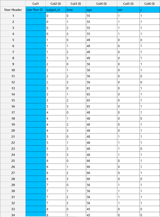
Configuration
- Select
Analytics\(\rightarrow\)Classification\(\rightarrow\)Statistical fitting\(\rightarrow\)Generalized Estimating Equations. - Set the
Type[1] of classification to Probit. - Specify the
Confidence Level (%)[2] for the test. - Specify
Max Iterations[3]. - Specify
Iterations Between Updates[4]. - Select the
Dependent Variable[5]. - Select the
Reference Category[6]. - Specify the
Minimum Change in Parameter Estimates[7]. - Specify the
Hessian Convergence[8]. - Specify the
Scale Parameter[9]. - Select the
Within Subject[10]. - Select the
working correlation Structureand specify the value ofMif you select M-Dependent as the correlation structure. [11]. - Select the method used to estimate the
covariance matrix[12] of the standard errors. - Select the columns by clicking on the arrow buttons [17] and moving columns between the
Excluded Columns[13] andSubjects[14] andFactors[15] andCovariates[16] lists. Specify Reference Levels[18] for the categorical factors.- Select the prefered
Formula Type[19]. Specify Custom Model Formula[20] for the analysis ifCustomoption is selected. How to specify a custom model formula?- Click on the
Executebutton [21] to perform the Probit Classification method.
Output
The Predictions, Parameter Estimates table and Working Correlation Matrix are shown in the output spreadsheet.
Complementary Log-Log
Use the Complementary Log-Log Classification method by browsing in the top ribbon:
| Analytics \(\rightarrow\) Classification \(\rightarrow\) Statistical fitting \(\rightarrow\) Generalized Estimating Equations |
And then choosing “Complementary Log-Log” as the Type.
Input
All variables must be specified in the datasheet. The dependent variable must be a binary categorical variable, containing exactly two distinct outcomes (e.g., 0 and 1, or two unique labels). The dependent variable should not contain missing entries or values outside the two defined categories. Independent variables may be either numerical or categorical. Categorical variables can be represented using either text labels or numerical codes. The input datasheet must include at least two columns: one for the dependent variable and one or more for the independent variables. Each row should represent a single observation. This model is particularly useful when the probability of the event is highly skewed (close to 0 or 1) and is often applied in contexts involving time-to-event outcomes or hazard-based modeling.
Configuration
| Confidence Level (%) | Specify the confidence level of the analysis. Values should range from 0 to 100 and correspond to percentages. |
| Max Iterations | Defines the maximum number of iterations the model is allowed to perform during the estimation process. If the model fails to converge before reaching this number, the algorithm stops and returns the values of the last iteration. |
| Iterations Between Updates | Defines how often the working correlation matrix is updated during estimation. |
| Dependent Variable | Select the column that corresponds to values of the dependent variable. |
| Reference Category | Specifies which category of the dependent variable should be used as the reference level when calculating parameter estimates. |
| Minimum Change in Parameter Estimates | Sets the tolerance level for convergence — the smallest change in parameter estimates between iterations required to continue optimization. If the change in all parameters is below this value, the algorithm assumes convergence has been reached. |
| Hessian Convergence | Specifies a threshold for convergence based on the second derivatives (Hessian matrix). |
| Scale Parameter | Adjusts the variance of the model. |
| Within Subject | Selects the column that defines the ordering of repeated observations within each subject. |
| Structure | Defines the working correlation structure for repeated measurements within subjects. Choices include Independent, Exchangeable, AR(1), Unstructured and M-Dependent. |
| M | In the M-Dependent correlation structure, M specifies the maximum number of consecutive observations within each cluster that are assumed to be correlated, with correlations set to zero for observations more than M time points apart. M must be an integer in the range from 1 to (number of within-subject observations – 1). |
| Covariance Matrix | In the Covariance Matrix option, the user selects how the model’s standard errors will be estimated. The Robust estimator is resistant to misspecification of the correlation structure, while the Model-based estimator assumes the specified correlation is correct. |
| Subjects/Factors/Covariates/Excluded Columns | Select manually the columns that correspond to subjects, factors and the columns that correspond to covariates through the dialog window: Use the buttons to move columns between the Subjects, Factors and Covariates list and Excluded Columns list. Single-arrow buttons will move all selected columns. At least one covariate or factor column should be specified. Also, a column for the Subject is required. |
| Specify Reference Levels | Specify the reference level for each of the categorical factors specified. The default option for each factor is its last level. |
| Formula Type | These options refer to the terms that will be included in the model. The Custom option allows the user to input a formula defining the exact terms to be included. The Main Effects option allows the analysis of a model that only includes all main effects and finally, the Full Factorial option includes both all main effects and all possible interaction terms to build a full model. |
| Specify Custom Model Formula | Specify the model formula used for the analysis if the Custom option is selected. The formula is created in the Custom Formula Creation dialog window by selecting factors and covariates and adding interaction terms up to the required order. Main effects of the included columns are always part of the model and cannot be excluded. |
Output
The output of the Generalized Estimating Equations (GEEs) procedure is organized into three main sections: the Predicted Values Table, the Parameter Estimates Table and the Working Correlation Matrix.
- The Predicted Values Table shows the fitted values for the dependent variable on the specified model.
- The Parameter Estimates Table includes the estimated coefficients for the independent variables. Each row corresponds to a predictor and includes its coefficient, standard error, confidence interval, test statistic, degrees of freedom, and p-value.
- The Working Correlation Matrix displays the estimated correlations between repeated measurements of the same subject over time
Example
Input
The dataset must include a binary outcome variable coded as 0 and 1, suitable for modeling with a complementary log-log (cloglog) link function. Cloglog classification within the GEE framework is particularly appropriate for modeling asymmetric binary outcomes, such as rare events or time-to-event responses observed over discrete intervals. The dataset should also include at least one independent variable, which can be continuous or categorical, a subject identifier to define repeated measurements within clusters, and a within-subject time or measurement variable to indicate the order of observations. The data structure should support modeling within-cluster correlation under the binomial distribution assumption using the complementary log-log link function in the GEE framework
Configuration
- Select
Analytics\(\rightarrow\)Classification\(\rightarrow\)Statistical fitting\(\rightarrow\)Generalized Estimating Equations. - Set the
Type[1] of classification to Complementary Log-Log. - Specify the
Confidence Level (%)[2] for the test. - Specify
Max Iterations[3]. - Specify
Iterations Between Updates[4]. - Select the
Dependent Variable[5]. - Select the
Reference Category[6]. - Specify the
Minimum Change in Parameter Estimates[7]. - Specify the
Hessian Convergence[8]. - Specify the
Scale Parameter[9]. - Select the
Within Subject[10]. - Select the
working correlation Structureand specify the value ofMif you select M-Dependent as the correlation structure. [11]. - Select the method used to estimate the
covariance matrix[12] of the standard errors. - Select the columns by clicking on the arrow buttons [17] and moving columns between the
Excluded Columns[13] andSubjects[14] andFactors[15] andCovariates[16] lists. Specify Reference Levels[18] for the categorical factors.- Select the prefered
Formula Type[19]. Specify Custom Model Formula[20] for the analysis ifCustomoption is selected. How to specify a custom model formula?- Click on the
Executebutton [21] to perform the Complementary Log-Log Classification method.
Output
The Predictions, Parameter Estimates table and Working Correlation Matrix are shown in the output spreadsheet.
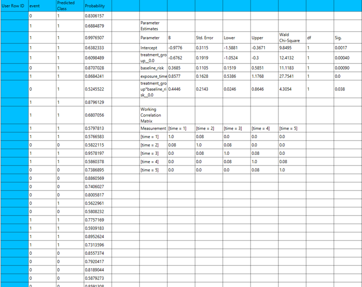
Ordinal Logistic
Use the Ordinal Logistic Classification method by browsing in the top ribbon:
| Analytics \(\rightarrow\) Classification \(\rightarrow\) Statistical fitting \(\rightarrow\) Generalized Estimating Equations |
And then choosing “Ordinal Logistic” as the Type.
Input
All variables must be specified in the datasheet. The dependent variable must be ordinal, coded as ordered categories (e.g., integers 1, 2, 3, …) and suitable for modeling with a cumulative logit (proportional odds) link function within the GEE framework for ordinal outcomes. Covariates should be numerical, while categorical predictors can be represented using either text labels or numeric codes. The input datasheet must include at least two columns: one for the dependent variable and one or more for the independent variables (covariates or factors). Each row should correspond to a single observation. Additionally, a subject identifier column is required to define clusters of repeated measurements, and optionally a within-subject variable to specify the order of observations within each subject. The structure of the dataset should support modeling intra-subject correlation under the multinomial/ordinal distribution assumption using the cumulative logit link within the GEE framework.
Configuration
| Confidence Level (%) | Specify the confidence level of the analysis. Values should range from 0 to 100 and correspond to percentages. |
| Max Iterations | Defines the maximum number of iterations the model is allowed to perform during the estimation process. If the model fails to converge before reaching this number, the algorithm stops and returns the values of the last iteration. |
| Iterations Between Updates | Defines how often the working correlation matrix is updated during estimation. |
| Dependent Variable | Select the column that corresponds to values of the dependent variable. |
| Minimum Change in Parameter Estimates | Sets the tolerance level for convergence — the smallest change in parameter estimates between iterations required to continue optimization. If the change in all parameters is below this value, the algorithm assumes convergence has been reached. |
| Hessian Convergence | Specifies a threshold for convergence based on the second derivatives (Hessian matrix). |
| Scale Parameter | Adjusts the variance of the model. |
| Within Subject | Selects the column that defines the ordering of repeated observations within each subject. |
| Structure | Defines the working correlation structure for repeated measurements within subjects. Choices include Independent, Exchangeable, AR(1), Unstructured and M-Dependent. |
| M | In the M-Dependent correlation structure, M specifies the maximum number of consecutive observations within each cluster that are assumed to be correlated, with correlations set to zero for observations more than M time points apart. M must be an integer in the range from 1 to (number of within-subject observations – 1). |
| Covariance Matrix | In the Covariance Matrix option, the user selects how the model’s standard errors will be estimated. The Robust estimator is resistant to misspecification of the correlation structure, while the Model-based estimator assumes the specified correlation is correct. |
| Subjects/Factors/Covariates/Excluded Columns | Select manually the columns that correspond to subjects, factors and the columns that correspond to covariates through the dialog window: Use the buttons to move columns between the Subjects, Factors and Covariates list and Excluded Columns list. Single-arrow buttons will move all selected columns. At least one covariate or factor column should be specified. Also, a column for the Subject is required. |
| Specify Reference Levels | Specify the reference level for each of the categorical factors specified. The default option for each factor is its last level. |
| Formula Type | These options refer to the terms that will be included in the model. The Custom option allows the user to input a formula defining the exact terms to be included. The Main Effects option allows the analysis of a model that only includes all main effects and finally, the Full Factorial option includes both all main effects and all possible interaction terms to build a full model. |
| Specify Custom Model Formula | Specify the model formula used for the analysis if the Custom option is selected. The formula is created in the Custom Formula Creation dialog window by selecting factors and covariates and adding interaction terms up to the required order. Main effects of the included columns are always part of the model and cannot be excluded. |
Output
The output of the ordinal logistic classification procedure is organized into three main sections: the Predicted Probabilities Table, the Parameter Estimates Table and the Working Correlation Matrix.
- The Predicted Probabilities Table displays the actual observed values of the ordinal dependent variable in the first column, followed by the predicted probabilities of each observation belonging to each outcome category. These probabilities are based on the fitted model and indicate how likely each case is to fall into each level of the ordinal outcome.
- The Parameter Estimates Table includes the estimated coefficients for the independent variables. Each row corresponds to a predictor and includes its coefficient, standard error, confidence interval, test statistic, degrees of freedom, and p-value.
- The Working Correlation Matrix displays the estimated correlations between repeated measurements of the same subject over time.
Example
Input
All variables must be specified in the datasheet. The dependent variable must be ordinal, coded strictly as numeric ordered categories (e.g., 1, 2, 3, …). The dataset must include at least one independent variable (continuous or categorical), a subject identifier to define repeated measurements, and optionally a within-subject time variable to indicate observation order. Each row should represent a single observation, and the data structure should support modeling intra-subject correlation under the ordinal distribution assumption using the cumulative logit link.
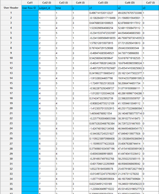
Configuration
- Select
Analytics\(\rightarrow\)Classification\(\rightarrow\)Statistical fitting\(\rightarrow\)Generalized Estimating Equations. - Set the
Type[1] of classification to Ordinal Logistic. - Specify the
Confidence Level (%)[2] for the test. - Specify
Max Iterations[3]. - Specify
Iterations Between Updates[4]. - Select the
Dependent Variable[5]. - Specify the
Minimum Change in Parameter Estimates[6]. - Specify the
Hessian Convergence[7]. - Specify the
Scale Parameter[8]. - Select the
Within Subject[9]. - Select the
working correlation Structureand specify the value ofMif you select M-Dependent as the correlation structure. [10]. - Select the method used to estimate the
covariance matrix[11] of the standard errors. - Select the columns by clicking on the arrow buttons [16] and moving columns between the
Excluded Columns[12] andSubjects[13] andFactors[14] andCovariates[15] lists. Specify Reference Levels[17] for the categorical factors.- Select the prefered
Formula Type[18]. Specify Custom Model Formula[19] for the analysis ifCustomoption is selected. How to specify a custom model formula?- Click on the
Executebutton [20] to perform the Ordinal Logistic Classification method.
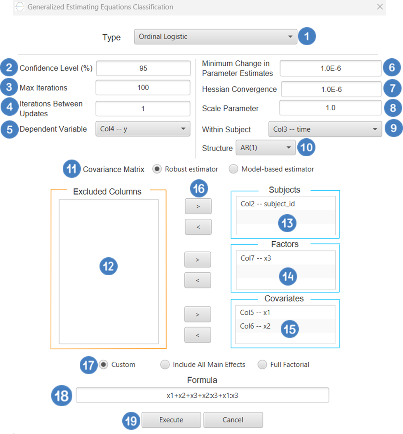
Output
The Predictions, Parameter Estimates table and Working Correlation Matrix are shown in the output spreadsheet.
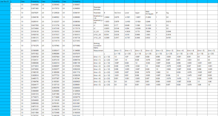
Ordinal Probit
Use the Ordinal Probit Classification method by browsing in the top ribbon:
| Analytics \(\rightarrow\) Classification \(\rightarrow\) Statistical fitting \(\rightarrow\) Generalized Estimating Equations |
And then choosing “Ordinal Probit” as the Type.
Input
All variables must be specified in the datasheet. The dependent variable must be ordinal, coded as ordered categories (e.g., integers 1, 2, 3, …) and suitable for modeling with a cumulative probit link function within the GEE framework for ordinal outcomes. Covariates should be numerical, while categorical predictors can be represented using either text labels or numeric codes. The input datasheet must include at least two columns: one for the dependent variable and one or more for the independent variables (covariates or factors). Each row should correspond to a single observation. Additionally, a subject identifier column is required to define clusters of repeated measurements, and optionally a within-subject variable to specify the order of observations within each subject. The structure of the dataset should support modeling intra-subject correlation under the multinomial/ordinal distribution assumption using the cumulative probit link within the GEE framework.
Configuration
| Confidence Level (%) | Specify the confidence level of the analysis. Values should range from 0 to 100 and correspond to percentages. |
| Max Iterations | Defines the maximum number of iterations the model is allowed to perform during the estimation process. If the model fails to converge before reaching this number, the algorithm stops and returns the values of the last iteration. |
| Iterations Between Updates | Defines how often the working correlation matrix is updated during estimation. |
| Dependent Variable | Select the column that corresponds to values of the dependent variable. |
| Minimum Change in Parameter Estimates | Sets the tolerance level for convergence — the smallest change in parameter estimates between iterations required to continue optimization. If the change in all parameters is below this value, the algorithm assumes convergence has been reached. |
| Hessian Convergence | Specifies a threshold for convergence based on the second derivatives (Hessian matrix). |
| Scale Parameter | Adjusts the variance of the model. |
| Within Subject | Selects the column that defines the ordering of repeated observations within each subject. |
| Structure | Defines the working correlation structure for repeated measurements within subjects. Choices include Independent, Exchangeable, AR(1), Unstructured and M-Dependent. |
| M | In the M-Dependent correlation structure, M specifies the maximum number of consecutive observations within each cluster that are assumed to be correlated, with correlations set to zero for observations more than M time points apart. M must be an integer in the range from 1 to (number of within-subject observations – 1). |
| Covariance Matrix | In the Covariance Matrix option, the user selects how the model’s standard errors will be estimated. The Robust estimator is resistant to misspecification of the correlation structure, while the Model-based estimator assumes the specified correlation is correct. |
| Subjects/Factors/Covariates/Excluded Columns | Select manually the columns that correspond to subjects, factors and the columns that correspond to covariates through the dialog window: Use the buttons to move columns between the Subjects, Factors and Covariates list and Excluded Columns list. Single-arrow buttons will move all selected columns. At least one covariate or factor column should be specified. Also, a column for the Subject is required. |
| Specify Reference Levels | Specify the reference level for each of the categorical factors specified. The default option for each factor is its last level. |
| Formula Type | These options refer to the terms that will be included in the model. The Custom option allows the user to input a formula defining the exact terms to be included. The Main Effects option allows the analysis of a model that only includes all main effects and finally, the Full Factorial option includes both all main effects and all possible interaction terms to build a full model. |
| Specify Custom Model Formula | Specify the model formula used for the analysis if the Custom option is selected. The formula is created in the Custom Formula Creation dialog window by selecting factors and covariates and adding interaction terms up to the required order. Main effects of the included columns are always part of the model and cannot be excluded. |
Output
The output of the ordinal probit classification procedure is organized into three main sections: the Predicted Probabilities Table, the Parameter Estimates Table and the Working Correlation Matrix.
- The Predicted Probabilities Table displays the actual observed values of the ordinal dependent variable in the first column, followed by the predicted probabilities of each observation belonging to each outcome category. These probabilities are based on the fitted model and indicate how likely each case is to fall into each level of the ordinal outcome.
- The Parameter Estimates Table includes the estimated coefficients for the independent variables. Each row corresponds to a predictor and includes its coefficient, standard error, confidence interval, test statistic, degrees of freedom, and p-value.
- The Working Correlation Matrix displays the estimated correlations between repeated measurements of the same subject over time.
Example
Input
All variables must be specified in the datasheet. The dependent variable must be ordinal, coded strictly as numeric ordered categories (e.g., 1, 2, 3,). The dataset must include at least one independent variable (continuous or categorical), a subject identifier to define repeated measurements, and optionally a within-subject time variable to indicate observation order. Each row should represent a single observation, and the data structure should support modeling intra-subject correlation under the ordinal distribution assumption using the cumulative probit link.
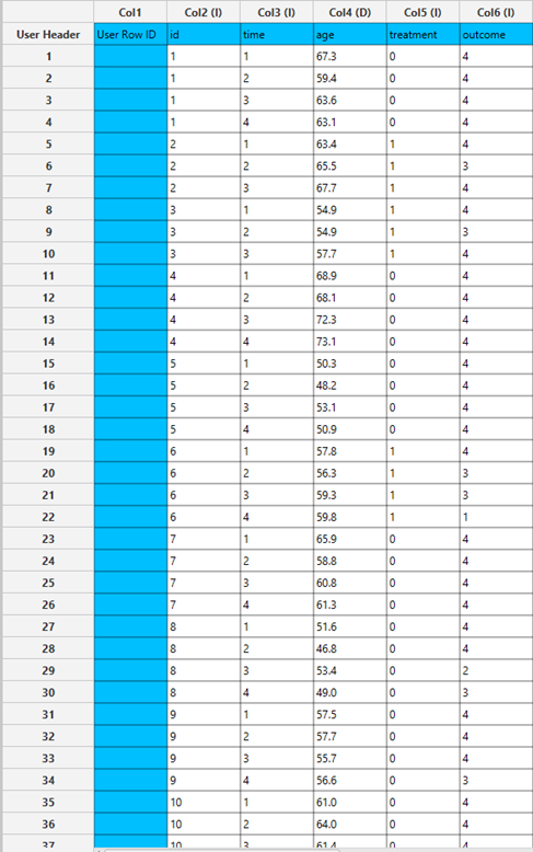
Configuration
- Select
Analytics\(\rightarrow\)Classification\(\rightarrow\)Statistical fitting\(\rightarrow\)Generalized Estimating Equations. - Set the
Type[1] of classification to Ordinal Probit. - Specify the
Confidence Level (%)[2] for the test. - Specify
Max Iterations[3]. - Specify
Iterations Between Updates[4]. - Select the
Dependent Variable[5]. - Specify the
Minimum Change in Parameter Estimates[6]. - Specify the
Hessian Convergence[7]. - Specify the
Scale Parameter[8]. - Select the
Within Subject[9]. - Select the
working correlation Structureand specify the value ofMif you select M-Dependent as the correlation structure. [10]. - Select the method used to estimate the
covariance matrix[11] of the standard errors. - Select the columns by clicking on the arrow buttons [16] and moving columns between the
Excluded Columns[12] andSubjects[13] andFactors[14] andCovariates[15] lists. Specify Reference Levels[17] for the categorical factors.- Select the prefered
Formula Type[18]. Specify Custom Model Formula[19] for the analysis ifCustomoption is selected. How to specify a custom model formula?- Click on the
Executebutton [20] to perform the Ordinal Probit Classification method.
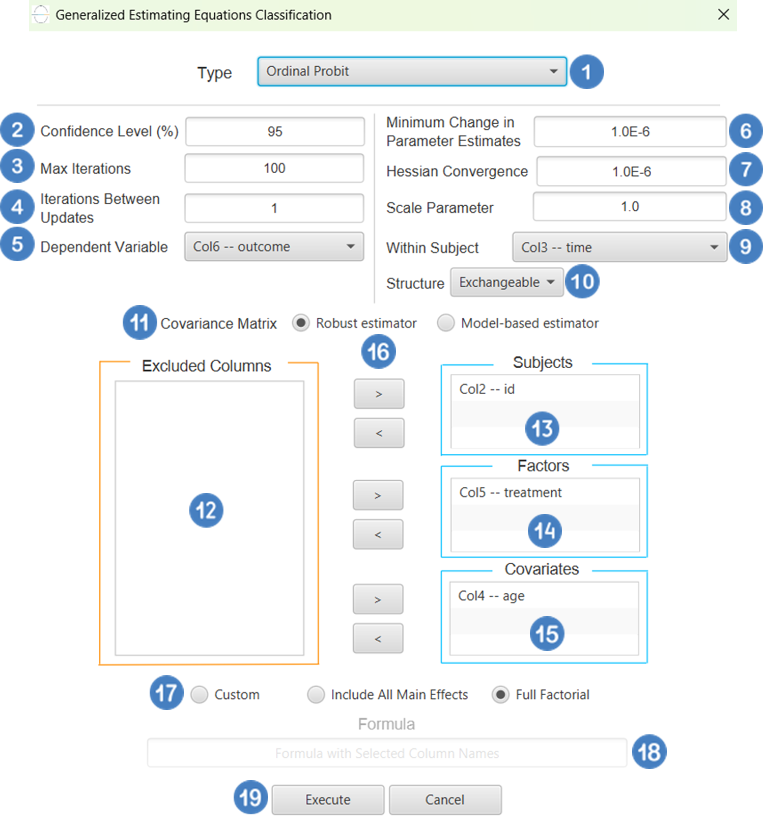
Output
The Predictions, Parameter Estimates table and Working Correlation Matrix are shown in the output spreadsheet.
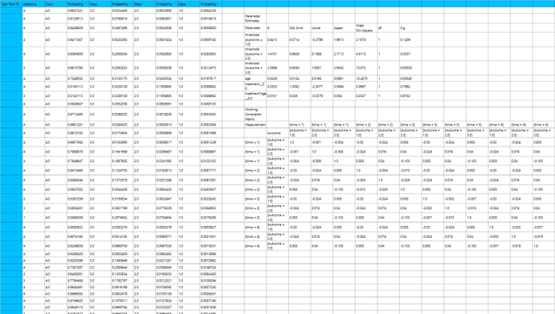
Auto ML
This function develops machine learning models for classification tasks and performs hyperparameter optimization to evaluate their performance. The models are trained and validated using all the variables of the input dataset after specification of the target variable. Additionally, the function supports multiple data splitting and normalization methods, as well as variable selection algorithms. Finally, all models are ranked according to the selected performance metrics.
Use the Auto ML function by browsing in the top ribbon:
| Analytics \(\rightarrow\) Classification \(\rightarrow\) Auto ML |
Input
Data matrix with training set data. The categories of the target feature should be presented as strings. Other categorical features must be encoded into numerical values, presented as either integers or doubles.
Configuration
| Available/selected models | Select manually the machine learning algorithms through the dialog window: Use the buttons to move algorithms between the Available Models and Selected Models list. Single-arrow buttons will move all selected algorithms and double-arrow buttons will move all algorithms. Available options include: k-Nearest Neighbours (kNN), Radial Basis Function Network, XGBoost, Random Forest, J48, and Fully Connected Neural Network. Double-click on each algorithm to specify the range (Min value, Max value and Step) of its hyperparameters. See more for the configuration options of each algorithm in the sections above. |
| RNG Seed | Select an integer as seed to get reproducible results. The option to select a time-based random number-generated seed is available. This seed will be used consistently for all operations within the AutoML function that require a seed. |
| Type | Select either Grid Search or the Genetic Algorithm to perform the hyperaparameter tuning. |
| Target column | Select manually from the drop-down menu the column name containing the target variable that is going to be predicted. |
| Split Method | Select manually from the drop-down menu the method for the splitting of the data into train and test sets. Available options include: Kennard-Stone, Random Partitioning, and k-Fold Partitioning. After you select the split method, specify its configuration parameters by clicking on Configure Split Method. See more for the configuration of each splitting method here. |
| Normalizer | Select manually from the drop-down menu a normalization method. Available options include: ZScore Normalizer and Min-Max Normalizer. If you select the Min-Max Normalizer, click on Configure Normalizer to specify the Min and Max values for the normalization. |
| Variable Selector | Select manually from the drop-down menu a variable selection method. Available options include: Genetic Algorithm, Boruta, Generalized Simulated Annealing, Particle Swarm Optimization, Recursive Feature Elimination, Successive Projections Algorithm, MI-VIF Variable Selection, and Best First. After you select the variable selection method, specify its configuration parameters by clicking on Configure Selector. See more for the configuration of each variable selection method here. |
| Selected Metric | Select manually from the drop-down menu the metric which will be used to evaluate the performance of each algorithm. Available options include: Accuracy, MCC, Confusion Matrix, Precision, Recall, F1Score, Sensitivity, False Discovery Rate, Youden’s J, Roc Auc, Hamming Loss, Balanced Accuracy, Kappa, Micro Precision, Macro Precision, Weighted Precision, Micro Recall, Macro Recall, Weighted Recall, Micro F1, Macro F1, Weighted F1, Micro Specificity, Macro Specificity, Weighted Specificity, Micro Youden’s J, Macro Youden’s J, Weighted Youden’s J, and Macro AverageRocAuc. |
| Top Results to Show | Specify how many of the algorithm ranking results, starting from the top, will be presented in the output speradsheet. |
| Number of Cores | Specify the number of CPU cores that will be used for the execution of the computations. |
Output
A ranking matrix of all the trained models including the number of top results specified in the Auto ML configuration box. The matrix presents the models starting from the top of the ranking, and consists of columns with each model’s algorithm, the variables used for the prediction of the target, and the evaluation metrics.
Example
Input
In the left-hand spreadsheet of the tab import the data matrix including the target variable, which should have at least two distinct categories for prediction. In case that categorical-string columns are included in the set, these should be encoded into representative numerical values.
Configuration
- Select
Analytics\(\rightarrow\)Classification\(\rightarrow\)Auto ML. - Select the algorithms by clicking on the arrow buttons and moving the algorithms between the
Available ModelsandSelected Modelslists [1]. - Double-click on each algorithm to specify the range of its hyperparameters. Default values, data types (double or integer) and acceptable ranges are indicated as guidance on the input parameter values [2], [3], [4].
- Type an
RNG Seed[5] for reproducible results or a random number generatedTime-based RNG Seed. - Select the
Typeof hyperparameter optimization methods [6]. - Select the
Target Columnthat is going to be predicted from the drop-down menu [7]. - Select the
Split Methodthat will be applied on the dataset from the drop-down menu [8]. - Click on
Configure Split Methodto specify the parameters of the splitting method [9], [10]. - Select a
Normalizer[11] from the drop-down menu. If you select the Min-Max nomralizer click onConfigure Normalizerto specify the minimum and maximum values for the normalization [12], [13]. - Select a method from the
Variable Selectordrop-down menu to remove redundant prediction variables [14]. - Click on
Configure Selectorto specify the parameters for the variable selection method [15], [16]. - Select the metric which will evaluate the model performance from the
Selected Metricdrop-down menu [17]. - Type the number of
Top Results to Showfrom the model ranking [18]. - Type the
Number or Coresthat will be used to execute the computations [19]. - Click on the
Executebutton to apply the Auto ML function [20].
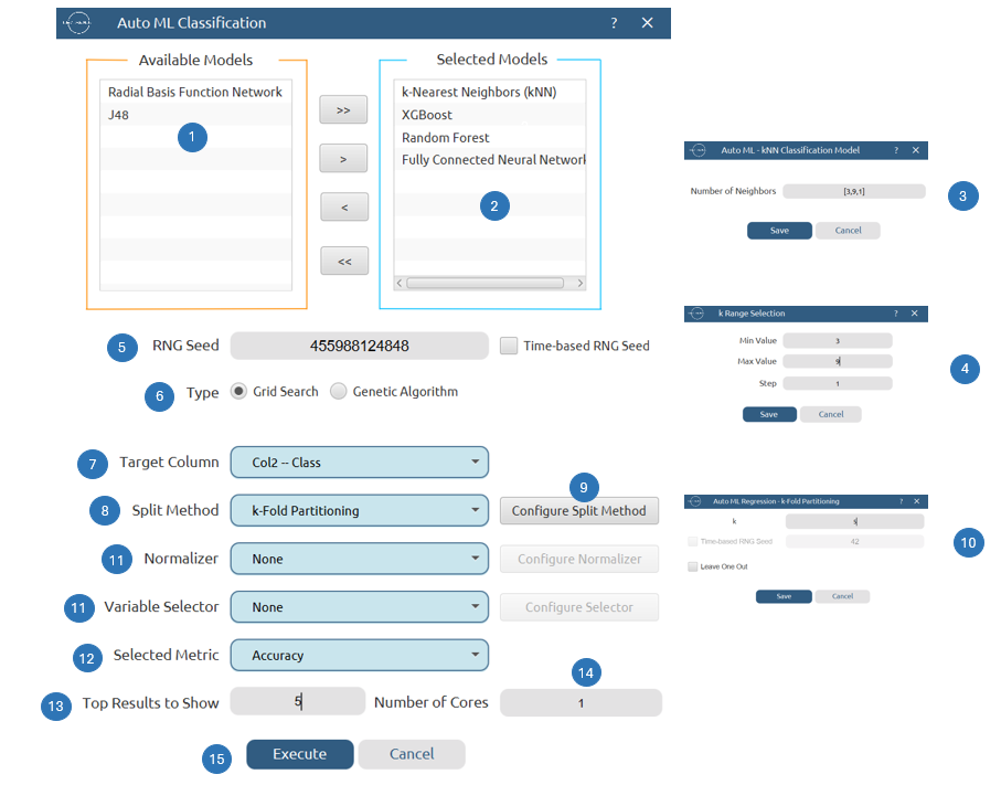
Output
In the right-hand spreadsheet of the tab the matrix with the ranking of the predictive models is presented.
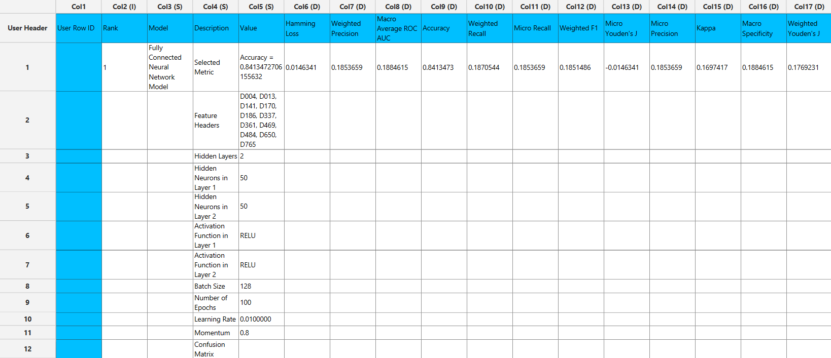
✧ Tips
- It works more efficiently for small to medium datasets and low-dimensional data. kNN is sensitive to missing data.
- The performance of the model is highly influenced by the selection of k.
- The number of neurons in the hidden layer has a high impact on the model performance, since a large number of neurons can lead to overfitting.
- Be cautious during hyperparameter tuning: choosing smaller
etavalues, as well as increasing thelambda,alpha, andgammavalues, result in a more conservative boosting process. Increasing the value of themax depthparameter makes the model more complex and more likely to overfit.
- This algorithm performs well with datasets that contain missing values. However, it is not as efficient with a large number of sparse features or with categorical variables of many levels that are improperly encoded.
See also
The model generated by any of the k Nearest Neighbors (kNN), Fully Connected Neural Network, Radial Basis Function Network, XGBoost, J48 Decision Tree, or Random Forest classification algorithms can be applied to any input data through the Existing Model Utilization function (e.g., a classification algorithm trained from the training set data of a machine learning model can be applied to the test/external set data).
References
- Witten Ian H and Frank, Eibe and Hall, Mark A and Pal CJ. Data Mining: Practical Machine Learning Tools and Techniques. Fourth. Morgan Kaufmann; 2011. https://doi.org/10.1016/C2009-0-19715-5.
- Murphy KP. Machine Learning: A Probabilistic Perspective. The MIT Press; 2012. 10.5555/2380985.
- Kohonen T. Self-organized formation of topologically correct feature maps. Biol Cybern 1982;43:59–69. https://doi.org/10.1007/BF00337288.
- Van Hulle MM. Self-organizing Maps. In: Rozenberg G, Bäck T, Kok JN, editors. Handbook of Natural Computing, Berlin, Heidelberg: Springer Berlin Heidelberg; 2012, p. 585–622. https://doi.org/10.1007/978-3-540-92910-9_19.
- Lee C-C, Chung P-C, Tsai J-R, Chang C-I. Robust radial basis function neural networks. IEEE Transactions on Systems, Man, and Cybernetics, Part B (Cybernetics) 1999;29:674–85. https://doi.org/10.1109/3477.809023.
- Ghosh J, Nag A. An Overview of Radial Basis Function Networks. In: Howlett RJ, Jain LC, editors. Radial Basis Function Networks 2: New Advances in Design, Heidelberg: Physica-Verlag HD; 2001, p. 1–36. https://doi.org/10.1007/978-3-7908-1826-0_1.
- XGBoost Parameters — xgboost 2.1.0-dev documentation n.d. https://xgboost.readthedocs.io/en/latest/parameter.html (accessed June 3, 2024).
- Hastie T, Tibshirani R, Friedman J. The Elements of Statistical Learning. New York, NY: Springer New York; 2009. https://doi.org/10.1007/978-0-387-84858-7.
- Chen T, Guestrin C. XGBoost: A Scalable Tree Boosting System. Proceedings of the 22nd ACM SIGKDD International Conference on Knowledge Discovery and Data Mining, 2016, p. 785–94. https://doi.org/10.1145/2939672.2939785.
- Salzberg SL. C4.5: Programs for Machine Learning by J. Ross Quinlan. Morgan Kaufmann Publishers, Inc., 1993. Mach Learn 1994;16:235–40. https://doi.org/10.1007/BF00993309.
- Breiman L. Random Forests. Machine Learning 2001;45:5–32. https://doi.org/10.1023/A:1010933404324.
- Nelder JA, Wedderburn RWM. Generalized linear models. J R Stat Soc A. 1972;135(3):370-84.https://doi.org/10.2307/2344614.
- McCullagh P, Nelder JA. Generalized linear models. 2nd ed. London: Chapman & Hall/CRC; 1989. https://doi.org/10.1201/9780203753736.
- McCullagh P. Regression models for ordinal data. J R Stat Soc B. 1980;42(2):109-42. https://doi.org/10.1111/j.2517-6161.1980.tb01109.x.
- Liang KY, Zeger SL. Longitudinal data analysis using generalized linear models. Biometrika. 1986;73(1):13-22. https://doi.org/10.1093/biomet/73.1.13.
- Piegorsch WW, Casella G. Complementary log regression for generalized linear models. Am Stat. 1992;46(3):199-200. https://doi.org/10.1080/00031305.1992.10475858.
Version History
Introduced in Isalos Analytics Platform v0.1.18
Instructions last updated on January 2025