Variable Selection
Variable Selection, also referred to as feature selection, is a process that confronts the problem of identifying and selecting the most relevant variables from the overall set of available variables. This crucial aspect of machine learning plays a significant role in improving model performance, reducing overfitting and enhancing interpretability by focusing on the most meaningful data. By eliminating irrelevant or redundant variables, variable selection not only simplifies the model’s structure but also reduces computational complexity, paving the way for faster training times and better generalization to unseen data.
Variable selection methods are generally split into the following subcategories:
-
The “filter” approaches: These methods select variables based on a priori information provided by the analyst, such as the Signal-to-Noise ratio or other statistical measures, irrespective of the machine learning algorithms used. They are, generally, computationally inexpensive and easy to implement but since they operate independently, they might miss data interactions that could be important for prediction.
-
The “wrapper” approaches: These methods evaluate the machine learning model’s performance on different subsets of variables. The evaluation is performed using a validation set, if available, or through cross-validation techniques to assess the model’s predictive accuracy. The wrapper methods consider how each feature influences the model, and they can be adapted to different model types and evaluation metrics, but using such methods is computationally expensive and may lead to overfitted models.
Best First
The Best First algorithm is a “wrapper” method used for feature selection, where subsets of features are evaluated using an evaluation function ($f(x)$). Each feature subset is represented as a node in a tree. Depending on the algorithm’s direction (forward, backward, or bidirectional), the children (neighboring subsets) of each node are generated accordingly through a process called expansion.
At each step of the algorithm, two lists are maintained:
- OPEN: Contains subsets of features that have been generated but not yet expanded.
- CLOSED: Contains subsets that have already been expanded.
The algorithm proceeds as follows: At each iteration the best evaluation value is selected from the OPEN list and the respective subset is transferred to the CLOSED list after being expanded to generate its neighbors. Then each neighbor is evaluated using $f(x)$ and compared to the current best subset. If any of the neighbors has a better evaluation value than the current best, then the current best is updated. All of the neighbors generated during expansion are added to the OPEN list.
The algorithm terminates when there are k consecutive expansions where no improvement to the best subset is observed. The parameter k is a user-defined input that determines the stopping criterion (#Nodes before termination).
The initialization of the algorithm and the expansion process depend on the selected direction:
- Forward Direction: The algorithm starts with the empty feature set and when expanding a subset, its neighbors are subsets that include all features of the current subset plus an additional feature.
- Backward Direction: The algorithm starts with the full feature set and when expanding a subset, its neighbors are subsets that include all features of the current subset except one.
- Bidirectional Direction: The algorithm starts with the empty feature set and when expanding a subset, neighbors are generated based on both forward and backward directions.
The evaluation function ($f(x)$) used in Isalos’ implementation of the algorithm is a metric called Merit which is computed as:
Where the subset $S$ contains $k$ features, $\overline{r_{cf}}$ is the average feature-class correlation and $\overline{r_{ff}}$ the average feature-feature intercorrelation:
Here $r_{f_i y}$ is the correlation between variable $i$ and the response variable and $r_{f_i f_j}$ is the correlation between variables $i$ and $j$.
The numerator of this metric (Eq. 1) can be interpreted as an indication of how predictive a group of features is while the denominator showcases how much redundancy there is among the features.
Use the Best First variable selection by browsing in the top ribbon:
| Data Transformation \(\rightarrow\) Variable Selection \(\rightarrow\) Best First |
Input
The data input should consist of numerical instances, without any missing values. There are no inherent limitations on the number of columns or rows.
Configuration
| Target Column | Choose the column that corresponds to the response variable. |
| Select Direction | Select any of the three available options (forward, backward, bidirectional) to adjust the initialization and the expansion process of the algorithm. |
| #Nodes before termination | Insert the #Nodes before termination to specify a stopping criterion for the algorithm. Acceptable values are only integers larger than 0. |
Output
Once the algorithm is completed, the output spreadsheet will be simplified to contain only two elements: the response variable and the best subset of features selected by the algorithm. These features represent the most relevant variables for predicting the response, as determined by the variable selection process.
Example
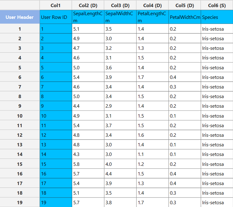
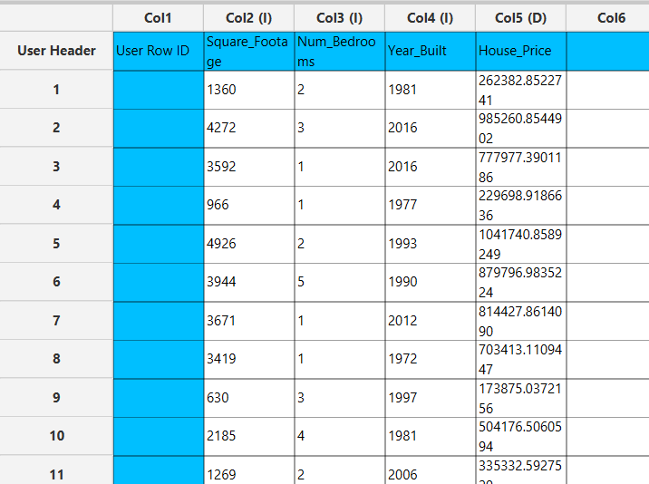
Input
In the left-hand spreadsheet of the tab import the data.
Configuration
- Select
Data Transformation\(\rightarrow\)Variable Selection\(\rightarrow\)Best First - Select the column that corresponds to the response variable as the
Target Column[1]. - Select one of the three available options for
Select Direction[2] to specify the initialization and expansion process of the algorithm. - Select
#Nodes before terminationto specify the stopping criterion of the algorithm [3]. - Click on the
Executebutton [4] to apply the methodology.

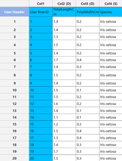
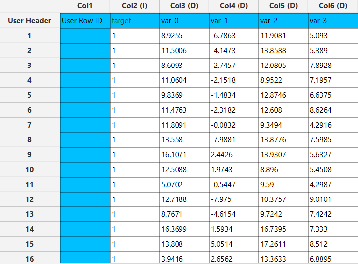
Output
The output data of the calculation is presented in the right-hand spreadsheet of the tab. It shows the dataset after the completion of Variable selection, meaning that it contains the response variable and the best subset of features selected by the algorithm.
Stepwise
Stepwise methods are “wrapper” methods used for regression models that analyze the significance of additional variables in a model, meaning that they compare the sum of squares of two models that differ only on the inclusion of one variable and decide whether the extra sum of squares is large enough to justify the inclusion of the additional value.
Consider the two models:
We denote the sum of squares due to regression as:
for models $M_1$ and $M_2$ respectively. The extra sum of squares due to the inclusion on $x_{k+1}$ is defined as $S_2 - S_1 = RSS_1 - RSS_2$, where $RSS$ is the residual sum of squares for each model. To test if the difference in the sum of squares is significant we estimate the variance as
and it can be shown that the test statistic $\frac{RSS_1-RSS_2}{\hat{\sigma}^2}$ follows the $F(1,N-(k+2))$ distribution which can be used to test whether the difference in sum of squares is statistically significant and therefore if the variable should be added to the model or not.
According to which method is chosen (Forward Selection, Backward Elimination) the algorithm proceeds as follows:
- Forward Selection: This forward selection starts with an empty model that only contains the intercept and then examines in each subsequent iteration the effect of including each of the remaining variables. This effect is evaluated according to a partial F-test as described above. The variable with the largest partial F-value is then included in the model. This selection process continues until none of the remaining variables has a partial F-value larger than a given critical value.
- Backward Elimination: The backward elimination method starts by building a model with all available variables. Subsequently, the effect of removing each of the variables in the model is evaluated according to a partial F-test as in the forward selection algorithm. The variable with the smallest partial F-value is then removed. This selection process continues until all variables in the model have partial F-values larger than a given critical value.
Use the Stepwise variable selection by browsing in the top ribbon:
| Data Transformation \(\rightarrow\) Variable Selection \(\rightarrow\) Stepwise |
Input
The data input should consist of numerical instances, without any missing values. There are no inherent limitations on the number of columns or rows.
Configuration
| Select Target Column | Choose the column that corresponds to the response variable. |
| Select Method | Select any of the two available options (Forward Selection , Backward Elimination) to choose which of the two methods to use. |
| Select Model | Select the type of regression model to be implemented (e.g. linear). |
| Threshold | Specify the critical value that will be used to compare F-values to decide whether the inclusion of a variable is significant. The values should range from 0 to 1. |
Output
Once the algorithm is completed, the output spreadsheet will be simplified to contain only two elements: the response variable and the best subset of features selected by the algorithm. These features represent the most relevant variables for predicting the response, as determined by the variable selection process.
Example
Input
In the left-hand spreadsheet of the tab import the data.
Configuration
- Select
Data Transformation\(\rightarrow\)Variable Selection\(\rightarrow\)Stepwise. Select Target Column[1] as the column that corresponds to the response variable.- Select one of the two available options for
Select Method[2] to specify which method to use. Select Model[3] to be implemented.- Specify the
Threshold[5]. Values should range from 0 to 1. - Click on the
Executebutton [5] to calculate the results.

Output
The output data of the calculation is presented in the right-hand spreadsheet of the tab. It shows the dataset after the completion of variable selection, meaning that it contains the response variable and the best subset of features selected by the algorithm.
Regression Analysis
Regression analysis is a “filter” method used to determine whether variables are linearly related to the response variable. This method constructs a linear regression model with the specified variables and evaluates measures such as R-squared, adjusted R-squared and the t-tests for each of the variables included in the model.
We denote as $\mathbf{X}$ the matrix that contains the data where each row of $\mathbf{X}$ corresponds to one instance of our sample space. We also denote as $C$, the matrix $C=(X^TX)^{-1}$. To perform a regression t-test for a specific variable we can test whether the linear coefficient of a feature is significantly different to zero with the following test:
Where $s^2=\frac{RSS}{N-k-1}$ is the sample variance, $\hat{b}_{j}$ is the estimator of the coefficient of the $j$-th variable and
$t_{N-k-1}$ is the student distribution with $N-k-1$ degrees of freedom.
A p-value is computed for each variable, which indicates whether its coefficient is statistically significantly different from zero. Variables with significant coefficients are deemed important and should be included in the model.
The user specifies a confidence level for the analysis, which is used to compute confidence intervals for each coefficient.
Use the Regression Analysis variable selection by browsing in the top ribbon:
| Data Transformation \(\rightarrow\) Variable Selection \(\rightarrow\) Regression Analysis |
Input
The data input should consist of numerical instances, without any missing values. There are no inherent limitations on the number of columns or rows.
Configuration
| Confidence Level (%) | Specify the confidence level of the analysis. Values should range from 0 to 100 and correspond to percentages. |
| Select Intercept Column | Choose the column that corresponds to the response variable. |
| Include/exclude columns | Select manually the columns to be included in the analysis through the dialog window: Use the buttons to move columns between the Included Columns and Excluded Columns list. Single-arrow buttons will move all selected columns and double-arrow buttons will move all columns. |
Output
Once the algorithm is completed, the output spreadsheet includes the results of the regression analysis: Metrics such as R-squared, Adjusted R-squared, the coefficients of each variable along with their test statistics, p-values, and confidence intervals, as well as the Analysis of Variance (ANOVA) table for the model.
Example
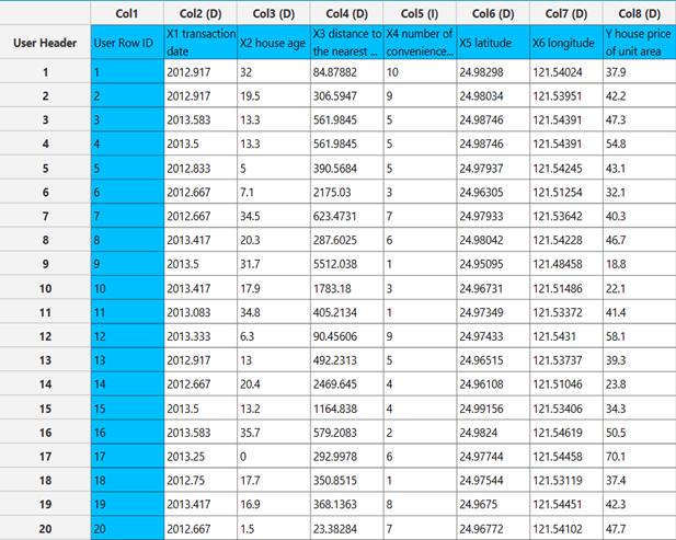
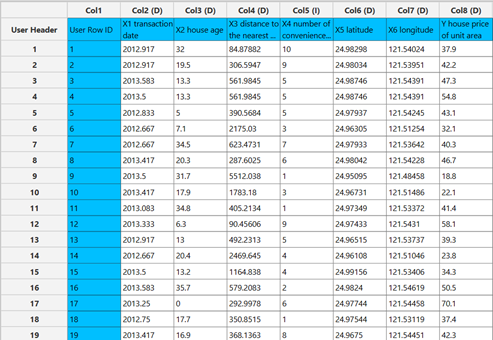
Input
In the left-hand spreadsheet of the tab import the data.
Configuration
- Select
Data Transformation\(\rightarrow\)Variable Selection\(\rightarrow\)Regression Analysis. - Specify the
Confidence Level (%)[1] for the test. Select Intercept Column[2] as the column that corresponds to the response variable.- Select the columns by clicking on the arrow buttons [4] and moving columns between the
Excluded Columns[3] andIncluded Columns[5] lists. - Click on the
Executebutton [6] to calculate the results.

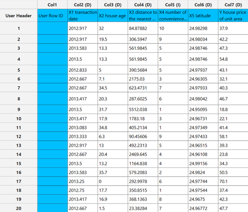
Output
The output data of the calculation is presented in the right-hand spreadsheet of the tab. The output includes the results of the regression analysis: Metrics such as R-squared, Adjusted R-squared, the coefficients of each variable along with their test statistics, p-values, and confidence intervals, as well as the Analysis of Variance (ANOVA) table for the model.
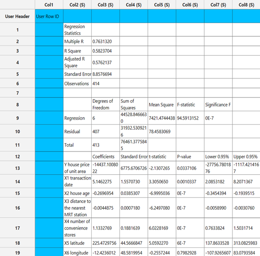
At a significance level of 0.05, the p-values of the coefficients indicate that the only variable that should be excluded from the set is “X6 (longitude),” as it is the only variable with a p-value greater than 0.05.
Genetic Algorithm
The Genetic Algorithm (GA) Variable Selection method is an evolutionary wrapper approach that identifies the optimal subset of input features to maximise predictive model performance. Inspired by the mechanisms of natural selection, the GA iteratively evolves a population of candidate feature subsets across multiple generations, guided by a fitness function that evaluates each candidate against a cross-validated model. GA-based selection belongs to the wrapper family of methods: each candidate subset is evaluated by actually training and testing a machine learning model, making the search intrinsically tied to the model’s predictive quality. 4
Each candidate solution (chromosome) is a binary string of length equal to the total number of input features. A bit value of 1 indicates that the corresponding feature is included in the subset; 0 means it is excluded. The algorithm searches this binary space to find the chromosome that yields the highest fitness.
When the number of GA evaluations (population size × generations) meets or exceeds the full search space size (2p, where p is the number of features), the algorithm automatically switches to exhaustive search, guaranteeing the globally optimal subset for small feature sets.
Automatic mode switching: If n × MAX ≥ 2p, an exhaustive multi-threaded search is performed instead of the GA, ensuring the best possible subset is returned without approximation.
Pre-processing
- The dataset is split according to the chosen splitter (e.g., k-fold, random).
- Each fold’s training data is normalised independently.
Evolutionary Search
- A population of n binary chromosomes is initialised with random 0/1 genes (p = 0.5 each).
- A new generation is created via:
- Single-point crossover
- Bit-flip mutation
- Tournament selection (size = 3) is used to choose which individuals reproduce.
- This process repeats for Max generations.
- The best chromosome overall is returned.
Fitness Function
For each candidate feature subset, the fitness is computed as the mean cross-validated metric across all folds, scaled by a factor that rewards smaller feature subsets:
\[fitness = \mathrm{metric} \cdot \left(1 + \lambda \cdot \frac{numOfFeatures - numOfSelectedFeatures}{numOfFeatures}\right)\]- metric — model performance (R² for regression or Classification Accuracy for classification)
- λ — weighting factor controlling the importance of feature reduction
- numOfFeatures — total number of available features
- numOfSelectedFeatures — number of selected features in the current chromosome
This formulation rewards high predictive performance while favouring smaller feature subsets.
Use the Genetic Algorithm variable selection function by browsing in the top ribbon:
| Data Transformation \(\rightarrow\) Variable Selection \(\rightarrow\) Genetic Algorithm |
Input
The data input should consist of numerical instances, without any missing values. There are no inherent limitations on the number of columns or rows.
Configuration
| Max Iterations | Define the maximum number of generations the GA will evolve. Combined with population size, this determines the total number of fitness evaluations: n × MAX. If this value equals or exceeds the full search space (2p), an exhaustive search is automatically performed instead. |
| Population Size | Specify a positive integer representing the number of candidate chromosomes evaluated per generation. Larger populations improve exploration of the feature space but increase computational cost per generation. |
| Crossover Probability | Specify the probability (0–1) that a pair of parent chromosomes undergoes crossover to produce offspring. If the probability is not met, both parents are copied unchanged into the next generation. Typical values range from 0.6 to 0.9. |
| Mutation Rate | Specify the probability (0–1) that any individual gene bit is flipped during mutation. A low mutation rate (e.g., 0.01–0.05) introduces small perturbations that help escape local optima without disrupting well-performing chromosomes. |
| Trade-off Factor (λ) | Define the weighting factor controlling the trade-off between predictive performance and feature reduction in the fitness function. Higher values place more emphasis on selecting fewer features. Typical values are small (e.g., 0.01–0.1). |
| Metric Selection | Choose whether the evaluation metric corresponds to a Regression or Classification problem. |
| Model Configuration | Select the model to use as the internal evaluator during the variable selection process. |
| Split Method | Choose the data splitting strategy used to evaluate each candidate feature subset. |
| Normalizer | Select a normalizer to apply to training and test data within each cross-validation fold prior to model training. |
| RNG Seed | Select an integer as seed to get reproducible results. The option to select a time-based random number-generated seed is available. |
| Target Column | Choose the column that corresponds to the response variable. |
Output
The algorithm returns the feature subset that achieved the highest fitness across all evaluated generations.
Example
Input
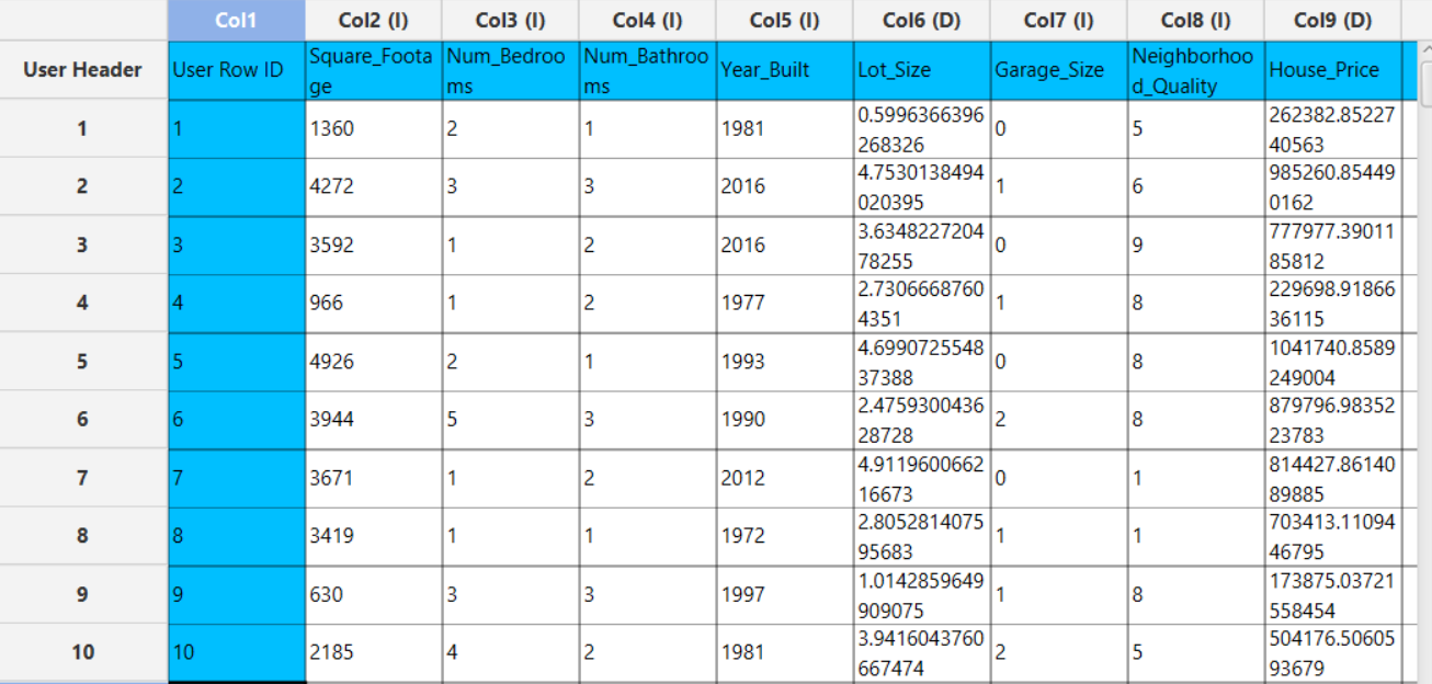
In the left-hand spreadsheet of the tab import the data.
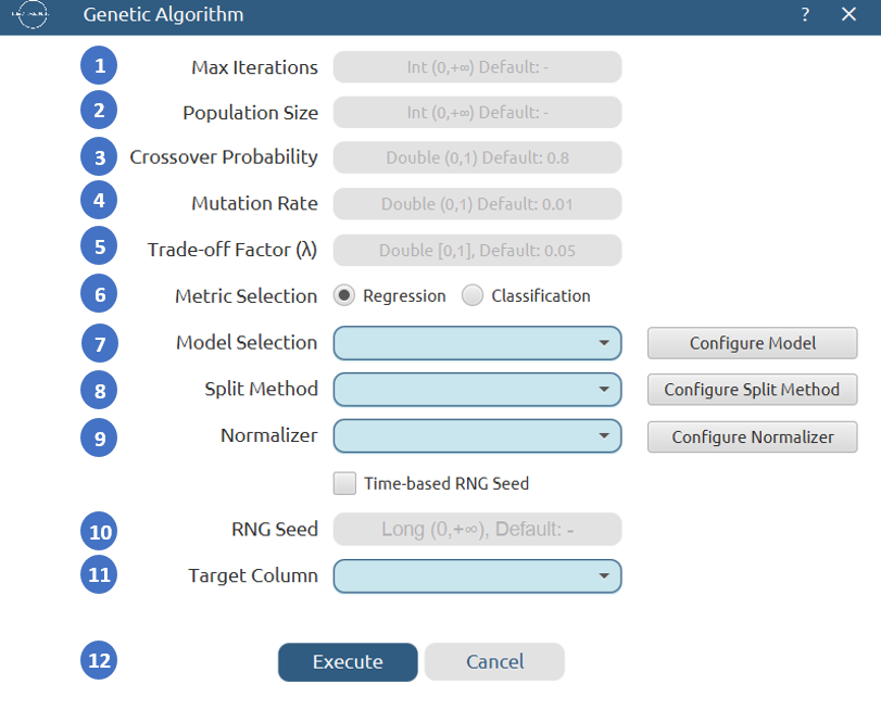
Configuration
- Select
Data Transformation\(\rightarrow\)Variable Selection\(\rightarrow\)Genetic Algorithm. - Set the
Max Iterations[1] andPopulation Size[2]. These jointly control the total number of fitness evaluations performed. - Set the
Crossover Probability[3] andMutation Rate[4]. - Set the
Trade-off Factor (λ)[5], which controls the trade-off between predictive performance and feature reduction. - Select the appropriate
Metric Selection[6] (Regression or Classification) depending on the nature of the problem. - Choose the predictive
Model Selection[7] to evaluate the candidate feature subsets and configure its parameters. - Select the
Split Method[8] to define the data splitting strategy. - Select the
Normalizer[9] to apply data preprocessing before model training. - Enable Time-based
RNG Seedor specify a fixed one [10] to ensure reproducibility. - Choose the
Target Column[11] to to be used for prediction. - Click the
Execute button[12] to run the algorithm.
Output
Once execution completes, the output will contain only the columns belonging to the best feature subset identified.
Successive Projections Algorithm
The Successive Projections Algorithm (SPA) is a geometry-driven wrapper method for variable selection that builds candidate feature chains by iteratively selecting the variable whose vector is most orthogonal to those already chosen. The resulting chains are then evaluated against a cross-validated model, and the subset yielding the best predictive performance is returned.
SPA does not rely on coefficient shrinkage or regularization. Instead, it selects variables iteratively by maximizing the projection of candidate variables onto the orthogonal subspace defined by the already selected variables. The objective is to reduce multicollinearity while preserving the most informative predictors for the target task. The method supports both regression and classification tasks. SPA is particularly well-suited for spectral and high-dimensional datasets where features are highly collinear, as the orthogonal projection step explicitly reduces redundancy.5
The algorithm runs in two parallel phases. In Phase 1, a separate feature chain is grown independently for every possible starting feature, producing p candidate chains (where p is the total number of features). In Phase 2, every prefix of every chain — is evaluated using cross-validated model performance. Both phases are parallelized. Finally, the subset with the highest score is selected.
Phase A: Projection-Based Variable Selection
Let xⱼ denote the j-th feature vector (column of matrix X).
For each of the p features as a starting point, a chain of numFeatures variables is constructed by iteratively selecting the feature whose projection onto the orthogonal complement of the already selected subspace has the largest norm. All p chains are built in parallel.
Orthogonal Projection Step
At each step, for every candidate feature vector xⱼ, the component orthogonal to the subspace spanned by the already selected features S is computed as:
\[\tilde{x}_j = x_j - P_S(x_j)\]where:
\[P_S(x_j) = \sum_{s \in S} \mathrm{proj}_{x_s}(x_j), \quad \mathrm{proj}_{x_s}(x_j) = \frac{x_j \cdot x_s}{\|x_s\|^2} \, x_s\]- xⱼ — feature vector across all samples
- S — set of selected feature indices
- x̃ⱼ — residual (orthogonal component)
The feature with the largest $|\tilde{x}_j|$ is selected.
Iterative Selection
At iteration k, given the selected set $S_{k-1}$:
\[r_j = x_j - P_{S_{k-1}}(x_j)\]The next feature is selected as:
\[j_k = \arg\max_j \|r_j\|\]Thus, at each step, the feature contributing the largest new orthogonal information is selected.
This process continues until a predefined number of variables is reached.
Phase B: Model Evaluation
After all chains are built, every prefix of every chain — a total of up to p × numFeatures candidate subsets — is evaluated independently and in parallel.
Regression subsets are scored by mean R² across folds. Classification subsets are scored by mean classification accuracy.
The subset yielding the highest mean cross-validated score across all chains and all prefix sizes is returned as the final selected feature set.
Use the Successive Projections Algorithm variable selection function by browsing in the top ribbon:
Use the Successive Projections Algorithm variable selection function by browsing in the top ribbon:
| Data Transformation \(\rightarrow\) Variable Selection \(\rightarrow\) Successive Projections Algorithm |
Input
The data input should consist of numerical instances, without any missing values. There are no inherent limitations on the number of columns or rows.
Configuration
| Max Number of Features | Specify the maximum chain length grown in Phase 1 and the maximum prefix size evaluated in Phase 2. |
| Metric Selection | Choose whether the evaluation metric corresponds to a Regression or Classification problem. |
| Model Selection | Select the type of regression/classification model to be implemented. |
| Split Method | Select the data splitting strategy |
| Normalizer | Select the normalization method to be applied to the dataset before model training |
| RNG Seed | Select an integer as seed to get reproducible results. The option to select a time-based random number-generated seed is available by clicking on the Time Based RNG Seed checkbox. |
| Target Column | Choose the column that corresponds to the response variable. |
Ouput
The algorithm returns the feature subset that achieved the highest score across all evaluated chains and prefix sizes.
Example
Input
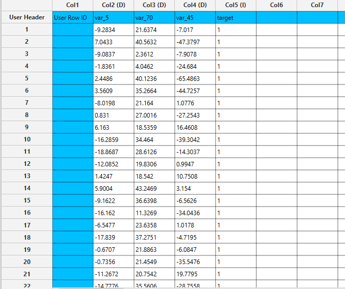
In the left-hand spreadsheet of the tab import the data.
Configuration
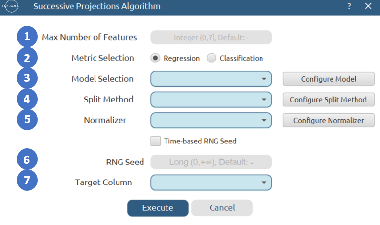
- Select
Data Transformation\(\rightarrow\)Variable Selection\(\rightarrow\)Successive Projections Algorithm. - Specify the
Max Number of Features[1]. - Select the appropriate
Metric Selection[2] (Regression or Classification) depending on the nature of the problem. - Choose the predictive
Model Selection[3] to evaluate the candidate feature subsets and configure its parameters if necessary. - Select the
Split Method[4] to define the data splitting strategy and configure its parameters if required. - Select the
Normalizer[5] to apply data preprocessing before model training. - Enable Time-based
RNG Seedor specify a fixed one [6] to ensure reproducibility. - Select the column that corresponds to the response variable as the
Target Column[7]. - Click on the
Execute button[8] to apply the methodology.
Output
Once execution completes, the output will contain only the columns belonging to the best feature subset identified.
Particle Swarm Optimization
Particle Swarm Optimization (PSO) is a “wrapper” method for feature selection inspired by the collective movement behaviour of biological swarms, such as flocks of birds or schools of fish. In the context of feature selection, a swarm of particles explores the feature space simultaneously, where each particle represents a candidate feature subset. Particles adjust their positions based on their own best-known solution and the best solution found by the entire swarm, gradually converging towards high-quality feature subsets.6
Algorithm Overview
The algorithm proceeds as follows:
Initialization: A swarm of $N$ particles is created, each with a randomly initialized position vector in $[0,1]^p$ and zero velocity. Each particle is evaluated and a set of non-dominated solutions is used to initialize the archive (leader set).
Iteration: At each iteration the following steps are applied:
-
Velocity update: Each particle’s velocity is updated based on its personal best position ($\mathbf{p}_i$) and a leader selected from the archive ($\mathbf{g}$):
\[\mathbf{v}_i^{t+1} = w \, \mathbf{v}_i^{t} + c_1 \, r_1 \, (\mathbf{p}_i - \mathbf{x}_i^{t}) + c_2 \, r_2 \, (\mathbf{g} - \mathbf{x}_i^{t}) \qquad [1]\]where $w$ is the inertia weight, $c_1$ and $c_2$ are acceleration coefficients, and $r_1$, $r_2$ are uniform random values in $[0, 1]$.
-
Position update: The particle’s position is updated as:
\[\mathbf{x}_i^{t+1} = \mathbf{x}_i^{t} + \mathbf{v}_i^{t+1} \qquad [2]\]Positions are clamped to $[0, 1]$.
-
Perturbation: Uniform and non-uniform mutation operators are applied to a fraction of the swarm to maintain diversity and escape local optima.
-
Evaluation: Each particle is evaluated by applying the 0.5 threshold to obtain a binary feature mask, training the selected model on the chosen features and computing the fitness value.
-
Archive update: The archive is updated with the current global best solution, and each particle’s personal best is updated if the new position improves its previous best.
The algorithm stops after a fixed number of iterations.
Fitness Function
For each candidate feature subset, the fitness is computed as the mean cross-validated metric across all folds, scaled by a factor that rewards smaller feature subsets:
\[fitness = \mathrm{metric} \cdot \left(1 + \lambda \cdot \frac{numOfFeatures - numOfSelectedFeatures}{numOfFeatures}\right)\]- metric — model performance (R² for regression or Classification Accuracy for classification)
- λ — weighting factor controlling the importance of feature reduction
- numOfFeatures — total number of available features
- numOfSelectedFeatures — number of selected features in the current chromosome
Use the Particle Swarm Optimization variable selection function by browsing in the top ribbon:
| Data Transformation \(\rightarrow\) Variable Selection \(\rightarrow\) Particle Swarm Optimization |
Input
The data input should consist of numerical instances, without any missing values. There are no inherent limitations on the number of columns or rows. Categorical features are excluded automatically prior to optimisation.
Configuration
| Max Iterations | Specify the number of iterations the swarm will run. Higher values allow more thorough exploration of the feature space but increase computation time. |
| Swarm Size | Define the number of particles in the swarm. Larger swarms explore more of the feature space per iteration but increase the computational cost per iteration. |
| Trade-off Factor (λ) | Define the weighting factor controlling the trade-off between predictive performance and feature reduction in the fitness function. Higher values place more emphasis on selecting fewer features. Typical values are small (e.g., 0.01–0.1). |
| Metric Selection | Choose whether the evaluation metric corresponds to a Regression or Classification problem. |
| Model Configuration | Select the model to use as the internal evaluator during the variable selection process. |
| Split Method | Choose the data splitting strategy used to evaluate each candidate feature subset. |
| Normalizer | Select a normalizer to apply to training and test data within each cross-validation fold prior to model training. |
| RNG Seed | Select an integer as seed to get reproducible results. The option to select a time-based random number-generated seed is available. |
| Target Column | Choose the column that corresponds to the response variable. |
Output
Once the algorithm is completed, the output spreadsheet will be simplified to contain only the response variable and the best subset of features selected by the algorithm.
Example
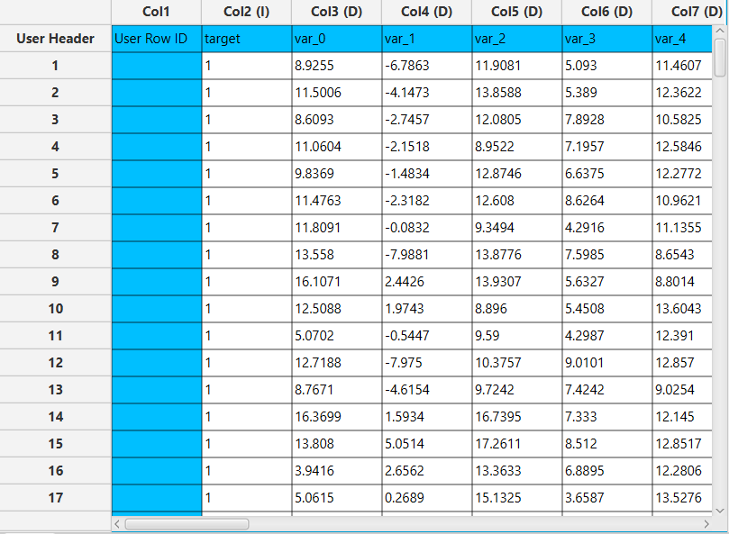
Input
In the left-hand spreadsheet of the tab import the data.
Configuration
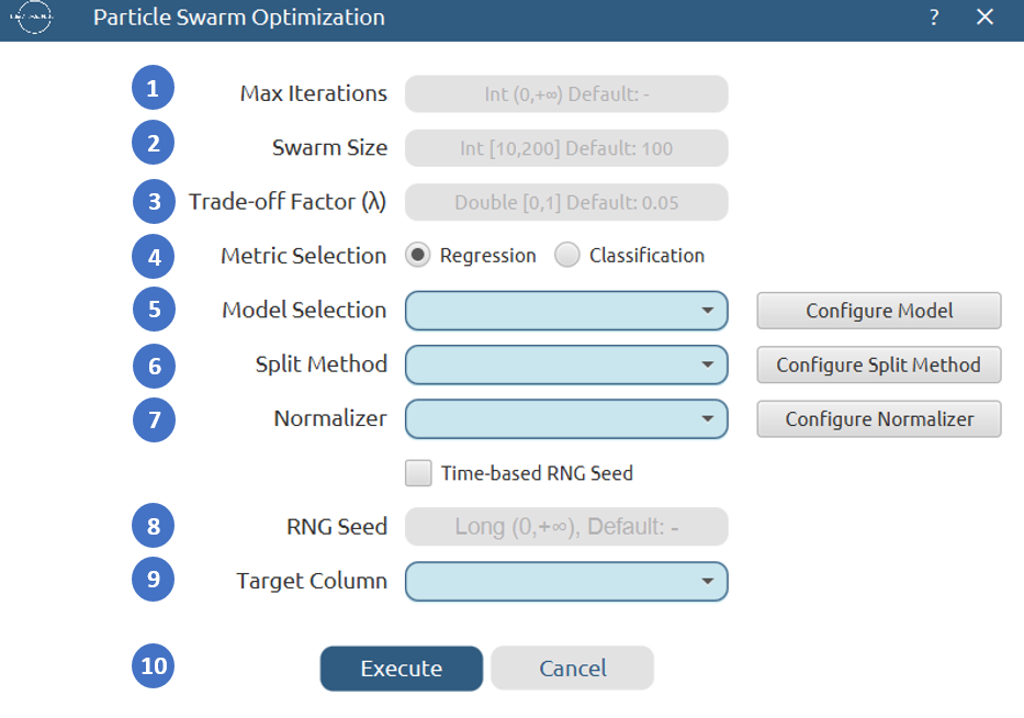
- Select
Data Transformation\(\rightarrow\)Variable Selection\(\rightarrow\)Particle Swarm Optimization. - Specify the
Max Iterations[1] to control how many iterations the swarm runs. - Specify the
Swarm Size[2] to set the number of particles. - Specify the
Trade-off Factor (λ)[3] to control the trade-off between accuracy and subset size. - Select the appropriate
Metric Selection[4] (Regression or Classification) depending on the nature of the problem. - Choose the predictive
Model Selection[5] to evaluate the candidate feature subsets and configure its parameters if necessary. - Select the
Split Method[6] to define the data splitting strategy and configure its parameters if required. - Select the
Normalizer[7] to apply data preprocessing before model training. - Enable Time-based
RNG Seedor specify a fixed one [8] to ensure reproducibility. - Select the column that corresponds to the response variable as the
Target Column[9]. - Click on the
Executebutton [10] to apply the methodology.
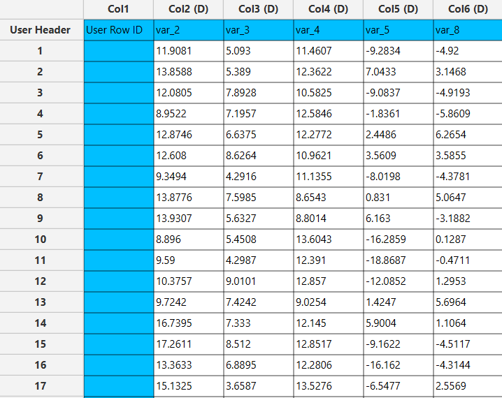
Output
Once execution completes, the output will contain only the columns belonging to the best feature subset identified.
Lasso
Lasso regression is an embedded variable selection method used to determine which predictor variables contribute significantly to the response variable. Unlike classical regression analysis that evaluates statistical significance through t-tests, LASSO performs variable selection by imposing an L1 regularization penalty on the regression coefficients. 7
This method constructs a linear regression model including all candidate variables and applies a sparsity constraint that shrinks some coefficients exactly to zero. Variables whose coefficients become zero are excluded from the model, while variables with non-zero coefficients are considered important predictors.
LASSO is primarily designed for regression tasks. However, it can also be applied to classification problems when the target variable is properly encoded. Encoding the target variable into numerical values allows the model to define a mathematical objective function, making it possible to apply LASSO regularization within classification models.
We denote by $X \in \mathbb{R}^{n \times p}$ the data matrix, where each row of Xcorresponds to one instance in the sample space and each column corresponds to one predictor variable. We denote by $y \in \mathbb{R}^{n}$ the response vector.
LASSO estimates the regression coefficients by solving the following optimization problem:
\[\hat{\beta} = \arg\min_{\beta} \left( \frac{1}{2n} \| y - X\beta \|^2 + \alpha \| \beta \|_1 \right)\]where:
- $\beta \in \mathbb{R}^p$ is the coefficient vector
- L1 norm: |β|₁ = Σ |βⱼ|
- $\alpha \geq 0$ is the regularization parameter
The regularization term α‖β‖₁ controls the sparsity of the solution.
As the value of α increases, more coefficients are forced toward zero.
After solving the optimization problem, the selected variables correspond to the indices j for which:
β̂ⱼ ≠ 0
Thus, feature selection is achieved directly through coefficient shrinkage.
The user specifies the regularization parameter α, which determines the trade-off between model fit and sparsity. Higher values of α increase sparsity by forcing more coefficients toward zero, resulting in fewer selected features. This approach is particularly effective in high-dimensional settings, where the number of predictors may be large relative to the number of observations.
Use the Lasso variable selection function by browsing in the top ribbon:
| Data Transformation \(\rightarrow\) Variable Selection \(\rightarrow\) Lasso |
Input
The data input should consist of numerical instances, without any missing values. There are no inherent limitations on the number of columns or rows.
Configuration
| Alpha | Specify the regularization parameter (α) controlling the strength of the L1 penalty. |
| Maximum Number of Features | Specify the maximum number of features to retain after selection. |
| Target Column | Choose the column that corresponds to the response variable. |
Output
Once the algorithm is completed, the output spreadsheet will be simplified to contain only two elements: the response variable and the subset of features with non-zero coefficients selected by the LASSO model. These features represent the most relevant predictors of the response variable, as determined by the L1-regularized regression process. Variables whose coefficients shrink to zero during optimization are automatically excluded from the final dataset.
Example
Input
In the left-hand spreadsheet of the tab import the data.

Configuration
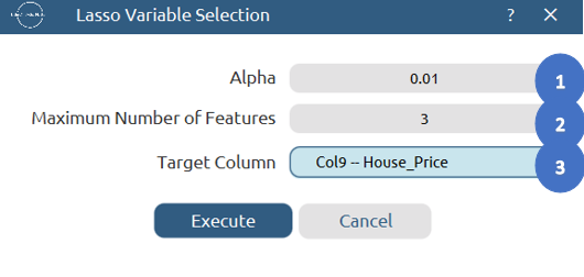
- Select
Data Transformation\(\rightarrow\)Variable Selection\(\rightarrow\)Lasso. - Specify the value of
Alpha[1] to control the strength of the L1 regularization. - Specify the
Maximum Number of Features[2] to limit the number of selected predictors. - Select the column that corresponds to the response variable as the
Target Column[3]. - Click on the
Executebutton [4] to apply the methodology.
Output
The output data of the calculation is presented in the right-hand spreadsheet of the tab. It shows the dataset after the completion of the LASSO variable selection process, meaning that it contains the response variable and only the features with non-zero coefficients selected by the algorithm.
MIVIF
The MI-VIF Variable Selection method is a two-stage filter approach that combines Mutual Information (MI) scoring with Variance Inflation Factor (VIF) filtering. Features are first ranked and thresholded by their statistical relevance to the target variable, then screened for multicollinearity. Only features that pass both criteria are retained.
Unlike wrapper methods such as the Genetic Algorithm, filter approaches evaluate features independently of any specific machine learning model, making MI-VIF computationally efficient and applicable to large datasets. The two-stage design addresses complementary problems: MI captures non-linear relevance between each feature and the target, while VIF detects and removes redundant features that are linearly explained by others already in the selected set.
Feature type (continuous vs. discrete) is detected automatically from the data distribution, and the appropriate MI estimator is selected per feature. This makes the method applicable without manual feature-type annotation.
Mutual Information Filtering
Each feature is scored against the target using a non-parametric MI estimator. Features with a score below the MI threshold are eliminated. The remaining features are ranked in descending order of MI score before proceeding to Phase 2.
Mutual information quantifies how much knowing one variable reduces uncertainty about another. It captures both linear and non-linear dependencies and equals zero if and only if two variables are statistically independent. Discrete features are detected automatically: a column is treated as discrete if the ratio of unique values to total samples is at or below 0.1 (i.e., fewer than 10% distinct values). All other features are treated as continuous.
The MI estimator is selected per feature based on the task type and the discreteness of the feature:
| Task | Feature type | Estimator | Method |
|---|---|---|---|
| Regression | Continuous | CC | KSG — continuous-continuous MI |
| Regression | Discrete | CD | Ross estimator — continuous target, discrete feature |
| Classification | Continuous | CD | Ross estimator — continuous feature, discrete target |
| Classification | Discrete | DD | Exact discrete-discrete MI (histogram) |
KSG Estimator (continuous–continuous)
The KSG estimator8 is a k-nearest-neighbour approach to estimating MI between two continuous variables. For each sample point, the Chebyshev distance to the k-th nearest neighbour in the joint space is used to define a radius; neighbour counts in each marginal space within that radius then enter the digamma-based estimator:
I(X; Y) = ψ(N) + ψ(k) − ⟨ψ(nₓ + 1) + ψ(nᵧ + 1)⟩
- ψ — digamma function
- N — total number of samples
- k — number of nearest neighbours (default: 3)
- nₓ, nᵧ — number of points within the k-th neighbour radius in each marginal
Prior to estimation, each variable is scaled by its population standard deviation and perturbed with tiny Gaussian noise to break ties.
Ross Estimator (continuous–discrete)
The Ross estimator9 handles the case where one variable is continuous and the other is discrete.
Within each class (discrete label), the k-th nearest neighbour distance is computed using the absolute distance on the continuous variable.
The estimator is defined as:
I(C; D) = ψ(N) − ⟨ψ(nₖ)⟩ + ψ(k) − ⟨ψ(m + 1)⟩
- N — total number of samples
- nₖ — size of the discrete class for sample i
- k — nearest neighbours within the class (capped at class size − 1)
- m — number of all samples within the within-class radius
Samples belonging to classes with only one member are excluded from the average.
Discrete–Discrete MI
When both the feature and the target are discrete, mutual information is computed exactly from the joint frequency table:
I(X; Y) = Σ p(x, y) · log( p(x, y) / (p(x) · p(y)) )
The summation is taken over all (x, y) pairs with non-zero joint probab
VIF Multicollinearity Filtering
Candidates from Phase 1 are evaluated one by one (highest MI first). Each candidate’s VIF is computed against the features already accepted. If VIF exceeds the threshold, the candidate is rejected; otherwise, it is accepted into the final set.
The Variance Inflation Factor (VIF) measures how well a feature can be linearly predicted from the features already accepted.
A high VIF indicates that the candidate feature carries information largely redundant with those already selected.10
VIF(Xⱼ) = 1 / (1 − R²ⱼ)
- R²ⱼ — coefficient of determination obtained by regressing feature Xⱼ on the currently accepted features using ordinary least squares (QR decomposition)
Interpretation:
- VIF = 1 — no correlation with other features
- VIF → ∞ — perfect collinearity (feature is rejected)
Typical thresholds:
- ≤ 5 — conservative
- ≤ 10 — more permissive
VIF Filtering Procedure
The filtering process evaluates features in descending order of mutual information (MI):
1. Select candidate
Pick the highest-MI feature not yet evaluated.
If no features have been accepted yet, set VIF = 1.0 and accept the feature.
2. Regress candidate on accepted features
Fit an OLS model (via QR decomposition using the internal LM solver) where the candidate is predicted from the accepted features.
Missing or infinite values are removed prior to fitting.
3. Compute R² and derive VIF
Compute R² from residuals and total sum of squares.
- If SST = 0 → VIF = 1.0
- If R² ≥ 1 − 10⁻¹² → VIF = ∞
4. Accept or reject
- If VIF ≤ threshold → accept the feature
- If VIF > threshold → reject the feature
5. Repeat
Continue until all MI-selected candidates have been evaluated.
Use the MI-VIF variable selection function by browsing in the top ribbon:
| Data Transformation \(\rightarrow\) Variable Selection \(\rightarrow\) MIVIF |
Input
A data matrix containing the input features and a target column.
Configuration
| MI Threshold | Specify the regularization parameter (α) controlling the strength of the L1 penalty. |
| VIF Threshold | Specify the maximum number of features to retain after selection. |
| Task type | Select Regression or Classification to determine how the target variable is treated during MI estimation. In regression mode the target is treated as continuous; in classification mode it is treated as discrete. This affects the MI estimator selected for each feature (see MI estimator routing table above). |
| Target Column | Choose the column that corresponds to the response variable. |
Output
The algorithm returns the subset of features that passed both the MI and VIF filters.
Example
Input
In the left-hand spreadsheet of the tab import the data.

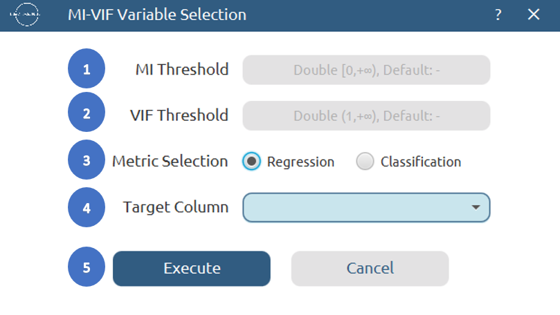
Configuration
- Select
Data Transformation\(\rightarrow\)Variable Selection\(\rightarrow\)MIVIF. - Set the
MI Threshold[1]. Features scoring below this value are eliminated before VIF evaluation. - Set the
VIF Threshold[2]. A value of 5.0 is a conservative starting point. - Select the
Task type[3]: Regression or Classification, depending on the nature of the target variable. - Select the column that corresponds to the response variable as the
Target Column[4]. - Click on the
Executebutton [5] to apply the algorithm on the input dataset.
Output
The right-hand spreadsheet will contain only the columns belonging to the final selected feature subset.
✧ Tips
- Ensure your dataset is preprocessed correctly before applying feature selection.
- Different evaluators and configurations may yield different results; experiment to find the best setup for your specific dataset and problem.
See also
Explore further preprocessing steps in the Data Transformation group of functions.
References
- Hall, Mark A. Correlation-based feature selection of discrete and numeric class machine learning. Proceedings of the Seventeenth International Conference on Machine Learning; 2000: 359–366. https://researchcommons.waikato.ac.nz/entities/publication/b2a8891e-8765-41fa-900d-10ca6258f29d.
- Kohavi, Ron, and George H. John. Wrappers for feature subset selection. Artificial intelligence 97.1-2; 1997: 273-324. doi.org/10.1016/S0004-3702(97)00043-X.
- Galvão, Roberto Kawakami Harrop, Mário César Ugulino de Araújo, and Sófacles Figueredo Carreiro Soares. Variable selection. In S. Brown, R. Tauler, & R. Walczak (Eds.), Comprehensive Chemometrics (Vol. 3, pp. 233–283). Oxford: Elsevier.
- Leardi, R.; Boggia, R.; Terrile, M. Genetic algorithms as a strategy for feature selection. Journal of Chemometrics 1992, 6(5), 267–281. https://doi.org/10.1002/cem.1180060506.
- Araújo, M. C. U.; Saldanha, T. C. B.; Galvão, R. K. H.; Yoneyama, T.; Chame, H. C.; Visani, V. The successive projections algorithm for variable selection in spectroscopic multicomponent analysis. Chemometrics and Intelligent Laboratory Systems 2001, 57(2), 65–73. https://doi.org/10.1016/S0169-7439(01)00119-8.
- Sierra, M.R., Coello Coello, C.A. Improving PSO-based multi-objective optimization using crowding, mutation and ∈-dominance. Evolutionary Multi-Criterion Optimization (EMO 2005). Lecture Notes in Computer Science, vol 3410. Springer, Berlin, Heidelberg. doi.org/10.1007/978-3-540-31880-4_35.
- Tibshirani, R. Regression shrinkage and selection via the lasso. Journal of the Royal Statistical Society: Series B (Methodological) 1996, 58(1), 267–288. https://doi.org/10.1111/j.2517-6161.1996.tb02080.x.
- Kraskov, A.; Stögbauer, H.; Grassberger, P. Estimating mutual information. Physical Review E 2004, 69(6), 066138. doi.org/10.1103/PhysRevE.69.066138.
- Ross, B. C. Mutual information between discrete and continuous data sets. PLOS ONE 2014, 9(2), e87357. doi.org/10.1371/journal.pone.0087357.
- Harel, Ofer (2009). The estimation of R2 and adjusted R2 in incomplete data sets using multiple imputation. Journal of Applied Statistics, 36(10), 1109-1118. https://doi.org/10.1080/02664760802553000.
Version History
Introduced in Isalos Analytics Platform v0.3.2
Instructions last updated on March 2025