Basic Statistics
Basic statistics is a tool that includes fundamental techniques used to summarize and interpret a given dataset. It encompasses descriptive statistics, such as mean, median, mode, variance, and standard deviation, which help characterize the central tendency and variability of data sets. It also includes confidence intervals, providing a range within which population parameters are likely to fall, and hypothesis testing, which allows analysts to make inferences or decisions based on sample data. Additionally, weighting cases can be applied to adjust for the relative importance of different data points. These tools are essential for understanding data behavior and supporting informed decision-making in research and analysis.
Descriptive Statistics
Descriptive statistics is a collection of analytical methods used to effectively summarize or describe a given dataset. These methods involve various measures, including measures of central tendency (e.g., mean, median, and mode), as well as measures of variability (e.g., range, variance, and standard deviation). By employing descriptive statistics, one can quickly evaluate the distribution and patterns within a dataset without relying on additional assumptions. Descriptive statistics play a crucial role as they offer valuable insights about a dataset in a straightforward manner, without the necessity of graphical representation, which might not have been feasible when dealing with large datasets.1.
The available statistical measures in Isalos, applicable to both the population and to a sample of the population, include:
1. Sample Size & Counts
This section covers the foundational counting measures of a dataset, including the total number of observations, how frequently individual values appear, their sum, and the sum of squared deviations from the mean.
Size/Count (n)
The size or count is the total number of data points in the dataset, denoted as $n$. It is used as the denominator in many statistical formulas to calculate averages and variations. Both population and sample datasets use the same method for counting data points.
Frequency
Frequency ($f_{i}$) refers to the number of times a particular data point or value appears in a dataset. It is a simple yet fundamental measure used to describe the distribution of data values. The basic formula for frequency is:
where $f_{i}$ represents the frequency of the $i$-th value $x_{i}$.
Use the Descriptive Statistics function by browsing in the top ribbon:
| Statistics \(\rightarrow\) Basic Statistics \(\rightarrow\) Descriptive Statistics |
Sum
The sum is the total of all numerical values in a dataset, calculated as:
Here, $x_{i}$ represents each value in the dataset. The calculation is identical whether dealing with a sample or a population.
Sum of Squares
The sum of squares (SS) is the sum of squared differences from the mean.
For populations:
For samples:
This foundational calculation underpins variance and standard deviation.
2. Central Tendency
This section describes measures that identify the centre of a distribution, with the mean, median, mode, and midrange, each offering a different perspective on where data values tend to cluster.
Mean
The mean, often referred to as the average, is a measure of central tendency that sums all the numerical values in a dataset and divides by the count of the values. The equation for calculating the mean is:
For populations:
For samples:
Median
The median is the middle value of a dataset when ordered. The method does not vary between sample and population datasets.
If $n$ is odd, the median is the middle number calculated at position $p$ (where $p = \frac{n + 1}{2}$):
If $n$ is even, it is the average of the two middle numbers at positions $p$ and $p+1$ (where $p = \frac{n}{2}$):
Mode
The mode is the value that appears most frequently in a dataset. A dataset may have one mode, multiple modes, or no mode if no number repeats more frequently than others. This calculation is consistent for both population and sample data.
Midrange
The midrange (MR) is the average of the maximum and minimum values of the dataset, calculated as:
This calculation is the same for both sample and population data.
3. Dispersion / Spread
This section quantifies how spread out the data values are around the centre, through measures including standard deviation, variance, range, and mean absolute deviation, with distinctions made between population and sample calculations where relevant.
Standard Deviation
Standard deviation measures the spread of data around the mean.
For populations:
For samples:
The difference lies in the denominator, where $n-1$ (Bessel’s correction) is used for samples to provide an unbiased estimator.
Variance
Variance measures the average squared deviations from the mean.
For populations:
For samples:
The distinction is similar to that of standard deviation.
Range
The range is a measure of the spread between the maximum and minimum values in the dataset, calculated as:
This measure does not differ between population and sample data.
Mean Absolute Deviation
The mean absolute deviation (MAD) is the average of absolute deviations from the mean, providing a measure of variability.
For populations:
For samples:
Minimum
The minimum (min) is the smallest value in a dataset, defining the lower boundary of the data range. There is no distinction in calculation between a sample and a population for this measure.
Maximum
The maximum (max) is the largest value in a dataset, defining the upper boundary of the data range. Like the minimum, the calculation does not vary between a sample and a population.
4. Quartiles, UQR & Outliers
This section explains how data can be divided into four equal parts to understand its spread, and how the interquartile range is used to identify data points that fall unusually far from the bulk of observations.
Available methods:
- Inclusive: Quartiles are calculated by assuming that the minimum and maximum of the sample correspond to the $0\%$ and $100\%$ percentiles respectively. The position of the quartile is determined by the formula:
where $p$ is the corresponding percentile ($0.25$, $0.50$, or $0.75$). If the position is not an integer, linear interpolation is used between the two adjacent observations.
- Exclusive: Quartiles are calculated by theoretically excluding the extremes of the sample from the estimation process. The position is given by the formula:
When the position is not an integer, linear interpolation is applied here as well.
Quartiles
Quartiles divide the data into four equal parts. $Q1$ is the median of the lower half, $Q2$ is the median of the dataset, and $Q3$ is the median of the upper half. The method for calculating quartiles is consistent across sample and population data.
Interquartile Range
The interquartile Range (IQR) is the difference between the third and first quartiles ($Q3$ - $Q1$), measuring the middle 50% spread of the data. There is no variation in calculating IQR between samples and populations.
Outliers
Outliers are data points significantly distant from other observations. They are typically identified using the IQR; values below $Q1 - 1.5 \times IQR$ or above $Q3 + 1.5 \times IQR$ are considered outliers. This identification method applies equally to sample and population data.
5. Relative / Advanced Measures
This section presents normalised measures of variability, with the coefficient of variation, relative standard deviation, root mean square, and standard error of the mean, which are particularly useful for comparing dispersion across datasets with different scales or units.
Coefficient of Variation
The coefficient of variation (CV) is a standardized measure of dispersion of a probability distribution or frequency distribution.
For populations:
For samples:
This measure is useful because it allows comparison between distributions with different units or means.
Relative Standard Deviation
The relative standard deviation (RSD) is expressed as a percentage and describes the dispersion or variability relative to the mean of the data.
For populations:
For samples:
Root Mean Square
The root mean square (RMS) provides a measure of the magnitude of a set of numbers, typically used to calculate the standard deviation. It is calculated by taking the square root of the average of the squares of the numbers:
Standard Error of the Mean
The standard error of the mean (SEM) measures the accuracy with which a sample represents a population.
For populations:
For samples:
This formula is consistent for both population and sample datasets.
6. Distribution Shape
This section covers skewness and kurtosis, which describe the asymmetry and tail heaviness of a distribution respectively, with separate formulas provided for population and sample data.
Skewness
Skewness ($\gamma_1$) is a measure of the asymmetry of the probability distribution of a real-valued random variable. Positive skewness indicates a distribution with an asymmetric tail extending towards more positive values, and negative skewness indicates a tail that extends towards more negative values.
For populations:
For samples:
Kurtosis
Kurtosis ($\beta_2$) measures the “tailedness” of the probability distribution of a real-valued random variable. High kurtosis in a data set is an indicator of substantial outliers.
For populations:
For samples:
Kurtosis Excess
Excess kurtosis ($\alpha_4$) is calculated by subtracting 3 from the standard kurtosis measurement. This adjustment helps to compare the tails of the distribution to those of a normal distribution, which has a kurtosis of 3.
For populations:
For samples:
7. Normality Tests
Normality Tests are inferential statistical methods, used to determine whether the sample data is modeled by a normal (Gaussian) distribution. In general, two competing hypotheses are formulated, the null hypothesis ($H_0$) and the alternative hypothesis ($H_\alpha$). Under the null hypothesis ($H_0$), it is assumed that the data follow a normal distribution. In contrast, the alternative hypothesis ($H_\alpha$) rejects this assumption, suggesting that the data exhibit significant deviations from normality. To reach an objective decision, these tests rely on p-values as a measure of evidence against or in support of the null hypothesis. This section covers three stastistical tests to assess whether sample data follow a normal distribution, each suited to different sample sizes and sensitivity requirements.
Shapiro-Wilk
The Shapiro-Wilk (S-W) is the most popular and powerful test for normality, especially for small to medium datasets (usually $n < 50$ to $n < 2000$). The test statistic ($W$) calculates the ratio of the best linear unbiased estimate of the variance to the usual corrected sum of squares estimate. In simpler terms, it compares the actual sample data to a perfectly normal distribution. A value of $W = 1$ indicates that the sample data perfectly match a normal distribution. The further $W$ is from $1$ (with $W < 1$), the more the data significantly deviate from a normal distribution.
where
- $x_{(i)}$: The $i$-th smallest number in the sample (ordered data points).
- $x_{i}$: Individual sample values.
- $\overline{x}$: The sample mean.
- $a_{i}$: Constants generated from the means, variances, and covariances of standard normal order statistics.
Kolmogorov-Smirnov
The Kolmogorov-Smirnov (K-S) test is better suited for larger datasets (usually $n > 2000$). However, it tends to be very sensitive with very large samples, often detecting minor, insignificant deviations. This test uses the Lilliefors Correction, adjusting the K-S test for when also estimating the mean and variance from the data. The test statistic ($D$) measures the maximum absolute vertical distance between the sample’s empirical cumulative distribution function (ECDF) and the cumulative distribution function (CDF) of a theoretical normal distribution. A smaller $D$ value indicates that the sample data closely match a perfect normal distribution. A larger $D$ value represents a larger deviation from normality.
where
- $\sup_{x}$: The supremum (the greatest) of the set of absolute differences.
- $F_n(x)$: The empirical cumulative distribution function (ECDF) of your sample data, which represents the proportion of data points less than or equal to $x$.
- $F(x)$: The cumulative distribution function (CDF) of a theoretical normal distribution (with the same mean and standard deviation as your sample).
Anderson-Darling
The Anderson-Darling (A-D) test is a variation of the K-S test that puts more weight on the tails of the distribution. It is useful when detecting heavy or light tails is important, since it is highly sensitive to outliers and deviations at the extremes. The test statistic ($A^2$) is calculated based on the squared differences between the sample’s empirical cumulative distribution function (ECDF) and the expected normal distribution’s cumulative distribution function (CDF). It measures how closely the sample data follow the theoretical normal curve. A small $A^2$ value indicates that the sample data closely follow a normal distribution. A large $A^2$ value indicates that the sample data deviate significantly from a normal distribution.
where
- $n$: The sample size.
- $X_{i}$: The ordered data points (sorted from smallest to largest).
- $F$: The cumulative distribution function of the normal distribution
8. Plots
This section presents four visualisation tools along with their customisation options, for graphically exploring data distributions and identifying patterns and outliers.
Q-Q Plot
A Quantile-Quantile (Q-Q) plot is a graphical tool for assessing whether a dataset might have been drawn from a particular theoretical distribution (e.g. normal or Weibull). The method plots the ordered values (quantiles or percentiles) of the observed data against the equivalent (theoretical) quantiles of a reference distribution. When the data aligns with the chosen theoretical distribution, the points on the plot will generally fall along an approximate straight diagonal line. To choose the theoretical distribution, select from the dropdown list next to the Q-Q Plot the corresponding option.
- Straight line: The data match the theoretical distribution.
- S-Shape (Curve): The data has “heavy tails” (outliers on both ends) or “light tails” than the theoretical distribution.
- Bending at one end: If the points curve away from the straight line only at the top or bottom, it indicates that the data is skewed (asymmetrical).
- Stray points: Points that drift away at the very ends of the line often point to the presence of outliers in the dataset.
Chart customization
Upon executing the Q-Q Plot, the resulting chart will appear in a separate window. By right-clicking on the plot, the following customization options are available:
Customization
| Show Legend | Display a legend consisting of the curves’ names. | |
| Show Grid | Display grid lines in the background. | |
| X axis ticks | Select the number of horizontal grid line ticks from the drop-down menu. | |
| Y axis ticks | Select the number of vertical grid line ticks from the drop-down menu. | |
| Series Properties | Select the desired properties for each series of data plotted on the chart. | |
| Series Color | Select series color. | |
| Line | Show a line connecting the data points. | |
| Point | Show data points. | |
| Area | Show the area between the confidence bands. | |
| Background | Select the background color. |
Settings
| Plotting Positions Method | Select the method for generating the plotting positions (cumulative probabilities). | ||
| Hazen | $P = \frac{i - 0.5}{n}$ | Popular in engineering; provides the median of the plotting distribution. | |
| Blom | $P = \frac{i - 0.375}{n + 0.25}$ | Designed to yield approximately normal quantiles. | |
| Weibull | $P = \frac{i}{n + 1}$ | Most common for general applications; unbiased for uniformly distributed data. | |
| Confidence Bands Method | Select the method for calculating the confidence bands. | ||
| Pointwise | Calculates the standard error of the sample order statistics individually at each quantile, then computes intervals at each point. | Good for checking the variability of individual quantiles. | |
| Kolmogorov-Smirnov | Based on the inversion of the Kolmogorov-Smirnov test. Calculates simultaneous bands that are proportional to the K-S critical value around the theoretical line. | Recommended for testing overall goodness-of-fit. | |
| Beta | Calculates exact, simultaneous bands using the order statistics of a sample. By leveraging the Beta distribution, it estimates a probability interval for each ordered data point. | Best for identifying deviations, extreme skew, or heavy tails. |
Histogram
A Histogram is a bar chart-based visualization used to show the frequency distribution of continuous numerical data. It groups the data into equally sized, continuous intervals knows as bins, where the height of each bar indicates the number of observations that fall within that particular interval.
Chart customization
Upon executing the Histogram, the resulting chart will appear in a separate window. By right-clicking on the plot, the following customization options are available:
Customization
| Show Legend | Display a legend consisting of the curves’ names. | |
| Show Grid | Display grid lines in the background. | |
| X axis ticks | Select the number of horizontal grid line ticks from the drop-down menu. | |
| Y axis ticks | Select the number of vertical grid line ticks from the drop-down menu. | |
| Series Properties | Select the desired properties for each series of data plotted on the chart. | |
| Series Color | Select series color. | |
| Visible | Show a line connecting the data points. | |
| Background | Select the background color. |
Settings
| Numbers of Bins | Select the number of bins to split the data into. |
Box Plot
A Box Plot is a standardized graphical method for displaying the distribution of numerical data based on a five-number summary: the minimum, first quartile, median, third quartile, and maximum. It is especially useful for identifying data skewness, spread, and outliers.
It visualises data distributions through these quantities:
- Median ($Q_{2}$): The middle value of the dataset, represented by a line inside the box. Half of the data is above this value, and half is below.
- The Box (Interquartile Range - $IQR$): Represents the middle $50\%$ of your data. The bottom of the box is the first quartile ($Q_{1}$) and the top is the third quartile ($Q_{3}$).
- Whiskers: Lines extending from the box to the minimum and maximum non-outlier values, showing the variability outside the middle $50\%$.
- Outliers: Individual points plotted beyond the whiskers, representing data points that significantly differ from the rest of the dataset.
Chart customization
Upon executing the Box Plot, the resulting chart will appear in a separate window. By right-clicking on the plot, the following customization options are available:
Customization
| Show Legend | Display a legend consisting of the curves’ names. | |
| Show Grid | Display grid lines in the background. | |
| Vertical | Select the orientation of the box plot to be vertical. | |
| Horizontal | Select the orientation of the box plot to be horizontal. | |
| Show Mean | Display the mean of the dataset. | |
| Show Outliers | Display the outliers of the dataset. | |
| Show Data Points | Display the data points. | |
| Point Spread | Select the spread of the data with respect to each other. | |
| Numerical Axis Controls | Select the number of grid line ticks from the drop-down menu. | |
| Category Colors | Select the color of the box plot. | |
| Background | Select the background color. |
Violin Plot
A Violin Plot is a data visualization tool used for comparing probability distributions across datasets. Similarly to a box plot, it summarizes data characteristics but it enhances the display by incorporating the probability density at different values. While a box plot shows summary statistics (such as the median and the interquartile range), it does not give information about the clusters of the data within those ranges. A violin plot overcomes this by adding a smoothed, symmetrical outer shape that indicates where the values are more dense, offering a clearer view of the overall distribution shape.
Chart customization
Upon executing the Violin Plot, the resulting chart will appear in a separate window. By right-clicking on the plot, the following customization options are available:
Customization
| Show Legend | Display a legend consisting of the curves’ names. | |
| Show Grid | Display grid lines in the background. | |
| Show Box Plot | Display the box plot inside the violin plot. | |
| Show Data Points | Display the data points. | |
| Point Spread | Select the spread of the data with respect to each other. | |
| Numerical Axis Controls | Select the number of grid line ticks from the drop-down menu. | |
| Category Colors | Select the color of the violin plot. | |
| Background | Select the background color. |
Settings
| Smoothness | Select the level of smoothness to apply. |
Input
The input spreadsheet consists of multiple columns, each representing a distinct dataset on which descriptive statistics will be utilized.
Configuration
| List of statistics | Select the appropriate methods for conducting descriptive statistics analysis by clicking on the corresponding radio buttons. The available statistics are described above. |
| Select Type | Select from the dropdown list the option that describes whether the data represents a sample or population. |
Output
In the output sheet, descriptive statistics analysis is performed by applying selected statistical measures to each dataset represented in the input sheet. The results display the statistical measures alongside their corresponding datasets in the respective columns.
Example
Input
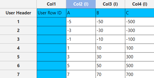
The input sheet on the left hand-side is organized with individual columns representing each data set. Insert the data sets in a manner that allows for independent analysis of each set when performing descriptive statistics.
Configuration
- Select
Statistics\(\rightarrow\)Basic Statistics\(\rightarrow\)Descriptive Statistics. - Determine whether the data correspond to
PopulationorSample[1] and click on the statistics that you wish to calculate for the input data [2]. - Click on the
Executebutton [3] to calculate the selected statistics.

Output
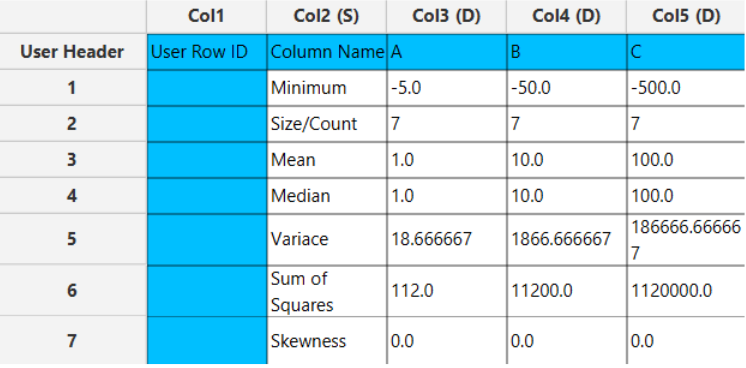
The right-hand side of the output sheet displays individual datasets per column, accompanied by the corresponding statistical measure chosen on each row.
Confidence Intervals
A confidence interval (CI) is a statistical tool used to estimate the range within which a population parameter (like a mean or proportion) is likely to fall, based on information from sample data1. This interval is constructed around the sample estimate and provides an indication of where the true parameter might be with a certain level of confidence, usually expressed as a percentage like 95% or 99%.2
To calculate a confidence interval, you typically need the sample mean (which provides a central estimate), the standard deviation (which measures the spread of the data), and the sample size (the number of data points). For proportions, you use the sample proportion instead of the mean. The formula for a confidence interval generally involves the sample statistic plus or minus a margin of error (Eq. 1), which is derived from the standard deviation and the sample size, adjusted by a factor from a statistical distribution (like the Z-score in large samples or the t-score in smaller samples)1,2.
The confidence interval when considering sample data is calculated based on the formula below:
where \(\begin{equation} \overline{x} \end{equation}\) is the sample mean, $s$ is the standard deviation of the sample data, $n$ is the sample data size and \(\begin{equation}t_{\text{critical}} \end{equation}\) is derived from the t-distribution, which accounts for degrees of freedom (df) that depend on the sample size and is found using Eq. 2 when confidence level is for example 95%:
where \(\begin{equation}df=n-1\end{equation}\) and $\alpha$ is the significance level which is calculated as \(\begin{equation}\alpha=1-\text{confidence level}\end{equation}\). The value \(\begin{equation}\frac{\alpha}{2}\end{equation}\) reflects the two-tailed nature of the typical confidence interval (e.g. for 95 % confidence interval, \(\begin{equation}\alpha=0.05\end{equation}\) and \(\begin{equation}\frac{\alpha}{2}=0.025\end{equation}\)).2
The confidence interval when considering population data is calculated based on Eq. 3:
Where $μ$ is the population mean, $σ$ is the standard deviation of the population data, $n$ is the population size and \(\begin{equation}Z_{\text{critical}}\end{equation}\) is derived from the standard normal distribution (Z-distribution), which is symmetric and has a mean of zero and a standard deviation of one. The \(\begin{equation}Z_{\text{critical}}\end{equation}\) value for a given confidence level is:
Where \(\frac{\alpha}{2}\) again accounts for the two-tailed nature of the test or interval. For a 95 % confidence interval, you look up or calculate the Z-value that corresponds to 97.5 % of the distribution (since 2.5 % is in each tail).2
The confidence interval when considering population proportion is calculated based on Eq. 5:
where $p$ is the sample proportion and is calculated as \(\begin{equation}p = \frac{X}{n}\end{equation}\): where X is the number of successes in the dataset and n is the total sample size.
Isalos offers three methods for calculating confidence intervals. The first method involves inputting raw (sample) data, assumed to be a representative sample. In this method, the mean can be automatically calculated, and the user has the option to manually input the standard deviation value or allow the software to calculate it automatically. This flexible approach allows for accurate estimation of confidence intervals based on the provided sample raw data. The second method requires the user to manually enter the mean value, standard deviation, and sample size. Additionally, the user must indicate whether the data represents a sample or population. The third method calculates confidence intervals based on proportions. Here, the user needs to specify the probability and sample size.
These different calculation options in Isalos provide flexibility and accommodate various scenarios for estimating confidence intervals with ease and accuracy. All the above three options allow the user to manually specify the confidence level.
Raw Data
As previously mentioned, the confidence intervals can be calculated using input raw (sample) data. The mean is automatically calculated, and the user has the option to manually enter or automatically calculate the standard deviation of the sample data. Additionally, the user can specify the desired confidence level for the calculation of the confidence intervals.
Use the Raw Data function for calculating confidence intervals by browsing in the top ribbon:
| Statistics \(\rightarrow\) Basic Statistics \(\rightarrow\) Confidence Intervals \(\rightarrow\) Raw Data |
Input
Users are allowed to input numerical values in any columns of their choice, without being constrained by specific limitations on the number of columns. It is important to note that the calculation will be rendered unable to be performed if categorical or text data is inserted.
Configuration
| Confidence level (α) | Manually insert confidence level which may range from 0 to 100. |
| Standard Deviation Method | Select any of the two options available, user-defined (Select by the user) or calculate the standard deviation based on the provided data (Autocalculate from input data). |
| Standard Deviation | If the previous option, Select by the user is chosen then enter manually the value that represents the standard deviation of the sample data. |
| Include/exclude columns | Select manually the columns that are going to be used for the calculation of the confidence interval through the dialog window: Use the buttons to move columns between the Included Columns and Excluded Columns list. Single-arrow buttons will move all selected columns and double-arrow buttons will move all columns. |
Output
The confidence interval is computed for each selected column, and the resulting values are presented in the output data sheet. Specifically, the lower limit is displayed in one row, while the upper limit is presented in another row.
Example
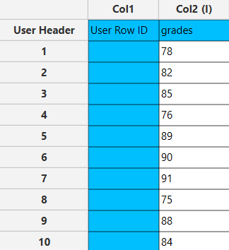
Input
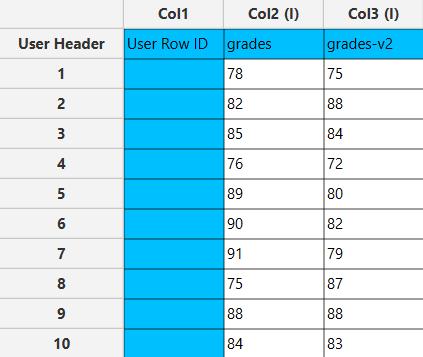
In the left-hand spreadsheet, each column specifies a data set for which we are interested in performing calculations for confidence intervals.
Configuration
- Select
Statistics\(\rightarrow\)Basic Statistics\(\rightarrow\)Confidence Intervals\(\rightarrow\)Raw Data. - Select
Confidence Level (α)[1]. The value will range from 0 to 100. - Select one of the two available options for the
Standard Deviation Method[2]: eitherAutocalculate from input dataorSelect by the user. If you choose the option toSelect by the user, enter the value of theStandard Deviation[3]. - Select the columns that are going to be used in the calculation by clicking on the arrow buttons [4] and moving columns between the
Excluded ColumnsandIncluded Columnslists. - Click on the
Executebutton [5] to apply the confidence intervals calculation on the selected columns.

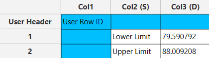
Configuration
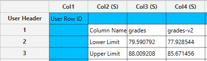
The output data of the calculation is presented in the right-hand spreadsheet of the tab, displaying the “Lower Limit” and “Upper Limit” for each selected column. These values indicate the range of the confidence interval.
Sample Size, Mean and Standard Deviation
This method offers the flexibility to the user to input the desired sample size, mean, and standard deviation, and to choose between sample data or population data representation. The user can also specify the confidence level.
Use the Sample Size, Mean and Standard Deviation function for calculating confidence intervals by browsing in the top ribbon:
| Statistics \(\rightarrow\) Basic Statistics \(\rightarrow\) Confidence Intervals \(\rightarrow\) Sample Size, Mean and Standard Deviation |
Input
No input data are needed to use this function.
Configuration
| Confidence level (α) | Manually insert confidence level which may range from 0 to 100. |
| Sample size (n) | Insert the number of data points in the dataset. |
| Mean ($\overline{\text{x}}$) | Type the mean value of the dataset. |
| Population/Sample | Select any of the two options available, σ or s that denotes that the dataset is population or sample data, respectively. |
| Standard Deviation | Type the value that represents the standard deviation of the data. |
Output
The output datasheet presents the Lower Limit and Upper Limit values in separate rows.
Example
Input
The left-hand spreadsheet contains a column that is populated with the necessary data for calculating the confidence interval.
Configuration
- Select
Statistics\(\rightarrow\)Basic Statistics\(\rightarrow\)Confidence Intervals\(\rightarrow\)Sample Size, Mean and Standard Deviation. - Type the
Confidence Level[1]. The value will range from 0 to 100. - Type the
Sample Size (n)[2]. - Type the
Mean ($\overline{\text{x}}$)[3]. - Select one of the two available options for the
Population/Sample[4]: eitherσorsthat denotes that the dataset is population or sample data, respectively. - Click on the
Executebutton [5] to apply the confidence intervals calculation.

Output
The output data of the calculation is presented in the right-hand spreadsheet of the tab, displaying the Lower Limit and Upper Limit.
Population Proportion
This method illustrates how the confidence interval provides a range of plausible values for the population proportion based on the sample data, factoring in the given level of confidence.
Use the Population Proportion function for calculating confidence intervals by browsing in the top ribbon:
| Statistics \(\rightarrow\) Basic Statistics \(\rightarrow\) Confidence Intervals \(\rightarrow\) Population Proportion |
Input
Ensure that the input datasheet contains only one column of data. The data should be of nominal type and are divided into distinct categories that are mutually exclusive. Examples of such categories include “yes” or “no” responses, “male” or “female” categories, “pass” or “fail” outcomes, etc. If integer values are used to represent these categories, such as 1 or 0, it is acceptable.
Configuration
| Confidence level | Manually insert confidence level which may range from 0 to 100. |
| Sample size (n) | Insert the number of data points in the dataset. |
| Possibility (p) | Enter the value that represents the sample proportion. |
Output
The output datasheet presents the Lower Limit and Upper Limit values in separate rows.
Example
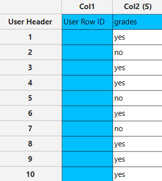
Input
The left-hand spreadsheet contains a column that is populated with the necessary data for calculating confidence intervals for a population proportion.
Configuration
- Select
Statistics\(\rightarrow\)Basic Statistics\(\rightarrow\)Confidence Intervals\(\rightarrow\)Population Proportion. - Type the
Confidence Level[1]. The value will range from 0 to 100. - Type the
Sample Size (n)[2]. - Type the
Possibility (p)[3]. - Click on the
Executebutton [4] to apply the confidence intervals calculation.

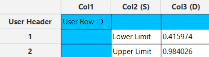
Output
The output data of the calculation is presented in the right-hand spreadsheet of the tab, displaying the Lower Limit and Upper Limit. This interval suggests that we are 95% confident that the true proportion of “yes” responses in the population lies between 41.6% and 98.4%.
Hypothesis Testing
Hypothesis testing is a statistical method used to decide whether the sample data sufficiently supports a particular hypothesis about a population. It generally involves formulating two competing hypotheses, the null hypothesis ($H_0$) and the alternative hypothesis ($H_a$), and then collecting data to assess the evidence. The null hypothesis ($H_0$) is the hypothesis that there is no effect or difference, and it assumes that any observed differences in the data are due to random chance. The alternative Hypothesis ($H_a$) is the hypothesis that challenges the null, proposing that there is a true effect or difference in the population.
The goal of hypothesis testing is to determine whether there is sufficient evidence to reject the null hypothesis. If the evidence is not strong enough, we fail to reject $H_0$, meaning the sample data does not provide enough proof against it.
The first step in hypothesis testing is to state the null and alternative hypotheses and then select a significance level ($a$) which represents the threshold for rejecting the null hypothesis, typically set at 0.05 (5%), meaning there’s a 5% chance of rejecting the null hypothesis when it is actually true (Type I error). Common values for $a$ are 0.05 (5%) and 0.01 (1%).
The next step involves choosing the test statistic. The test statistic depends on the nature of the data and the hypotheses being tested. Common test statistics include the Z-statistic (for large sample sizes or known population variance) and the t-statistic (for smaller sample sizes or unknown population variance).
For a Z-test:
For a t-test:
Where $\bar{x}$ is the sample mean, $\sigma$ and $s$ are the population and sample standard deviation respectively, $n$ is the sample size and $\mu_0$ is the assumed mean of the population under the null hypothesis.
After computing the test statistic, we follow up by either calculating the p-value or comparing the test statistic with a critical value. The p-value measures the probability of obtaining a test statistic at least as extreme as the one computed, assuming the null hypothesis is true. If the p-value is less than the chosen significance level ($a$), we reject $H_0$. In some cases, you compare the test statistic directly to a critical value derived from a statistical distribution ($Z$ or $t$). If the test statistic exceeds the critical value, reject $H_0$.
There are two main types of hypothesis tests:
- One-Tailed Test. This test assesses if the population parameter is either greater than or less than a specific value. For example:
- Two-Tailed Test. This test checks for any difference, whether positive or negative, from the hypothesized value. For example:
Isalos offers three methods for conducting hypothesis tests. The first method is called Sample Size, Mean and Standard Deviation and requires the user to input the sample size, the sample mean, select whether the standard deviation is known or calculated from the sample and give its value. The software then performs a Z-test if the population standard deviation is known or a t-test if it is unknown, based on the inputted hypotheses and significance level. The second method is called One Sample T-test and involves inputting raw (sample) data. In this method, the mean and the standard deviation are automatically calculated from the sample and then a t-test for the given hypotheses and significance level is performed. Finally, the last method is called One Sample Z-test, and also involves inputting raw (sample) data. Here, only the mean is automatically calculated from the sample, while the standard deviation is given from the user, and then a Z-test for the given hypotheses and significance level is performed.
These different hypothesis testing options in Isalos offer flexibility and can accommodate a variety of testing scenarios with ease and precision. All three methods allow the user to manually specify the significance level, ensuring accurate testing for a wide range of hypotheses.
Sample Size, Mean and Standard Deviation
This method offers the flexibility to the user to input the desired sample size, mean, and standard deviation, and to choose between known ($σ$) or unknown ($s$) standard deviation. The user can also specify the significance level and the hypotheses.
Use the Sample Size, Mean and Standard Deviation for conducting Hypothesis Testing by browsing in the top ribbon:
| Statistics \(\rightarrow\) Basic Statistics \(\rightarrow\) Hypothesis Testing |
And then in the Select Method option choose Sample Size, Mean and Standard Deviation.
Input
This method does not require any input in terms of raw (sample) data.
Configuration
| H$_0$: μ$_0$ | Manually insert the hypothesized mean. |
| H$_a$: μ$_a$ | Select any of the three options available for the alternative hypothesis (<, ≠, >). |
| Significance level (α) | Manually insert the significance level which may range from 0 to 1. |
| Sample size (n) | Insert the number of data points in the dataset. |
| Mean ($\bar{x}$) | Select the mean value of the dataset. |
| Standard Deviation Method | Select any of the two options available, Known StandardDeviation (σ) or Unknown StandardDeviation (s). |
| Standard Deviation | Type the value that represents the standard deviation of the data. |
Output
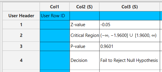
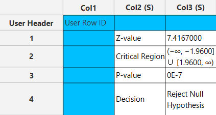
The hypothesis test is performed, and the output spreadsheet displays the test statistic, the critical region (region of rejection), the p-value, and the decision regarding the null hypothesis—whether it was rejected or not.
Example
Input
This method does not require any data to be inputted into the input spreadsheet.
Configuration
- Select
Statistics\(\rightarrow\)Basic Statistics\(\rightarrow\)Hypothesis Testing. - Select
Sample Size, Mean and Standard Deviationas the desired method [1]. - Manually insert the hypothesized mean [2]
- Select from the dropdown menu one of the three available options for the alternative hypothesis $H_a$ [3]: either
<,≠or>. - Select
Significance Level (α)[4]. The value will range from 0 to 1. - Type the
Sample Size (n)[5]. - Select
Mean ($\bar{x}$)[6]. - Select one of the two available options for the
Known Standard Deviation (σ)orStandard Deviation (s)[7] : either $σ$ or $s$ will be inputted, therefore will know if standard deviation is known from population or calculated from sample. - Type the
Standard Deviation[8]. - Click on the
Executebutton [9] to perform hypothesis testing.

Output
The output data of the calculation is presented in the right-hand spreadsheet of the tab. It shows the value of the test statistic, the critical region, the p-value of the test and the decision which is whether the null hypothesis was rejected or failed to be rejected.
One Sample T-test
This method allows the user to choose the null and alternative hypotheses and the significance level to perform an one sample T-test on raw data, that are stored in a single column.
Use the One Sample T-test method for performing hypothesis testing by browsing in the top ribbon:
| Statistics \(\rightarrow\) Basic Statistics \(\rightarrow\) Hypothesis Testing |
And then in the Select Method option choose One Sample T-test.
Input
This method only allows hypothesis testing for a single column therefore users should fill the desired column with numerical values and not nominal values.
Configuration
| H$_0$: μ$_0$ | Manually insert the hypothesized mean. |
| H$_a$: μ$_a$ | Select any of the three options available for the alternative hypothesis (<, ≠, >). |
| Significance level (α) | Manually insert the significance level which may range from 0 to 1. |
| Target Column | Select which column you want to perform hypothesis testing on. |
Output
The hypothesis test is performed, and the output spreadsheet displays the test statistic, the critical region (region of rejection), the p-value, and the decision regarding the null hypothesis—whether it was rejected or not.
Example
Input
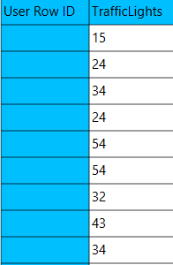
The left-hand spreadsheet contains a column that is populated with the necessary to perform the One Sample T-test on.
Configuration
- Select
Statistics\(\rightarrow\)Basic Statistics\(\rightarrow\)Hypothesis Testing. - Select
One Sample T-testas the desired method [1]. - Manually insert the hypothesized mean [2].
- Select one of the three available options for the alternative hypothesis $H_a$ [3]: either
<,≠or>. - Select
Significance Level (α)[4]. The value will range from 0 to 1. - Select the
Target column[5] to perform hypothesis testing on. - Click on the
Executebutton [6] to perform hypothesis testing.

Output
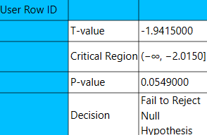
The output data of the calculation is presented in the right-hand spreadsheet of the tab. It shows the value of the test statistic, the critical region, the p-value of the test and the decision which is whether the null hypothesis was rejected or failed to be rejected.
One Sample Z-test
This method allows the user to specify the null and alternative hypotheses, the significance level of the test and the population’s standard deviation (σ) to perform an one sample Z-test on raw data, that are stored in a single column.
Use the One Sample Z-test method for performing hypothesis testing by browsing in the top ribbon:
| Statistics \(\rightarrow\) Basic Statistics \(\rightarrow\) Hypothesis Testing |
And then in the Select Method option choosing One Sample Z-test.
Input
This method only allows hypothesis testing for a single column therefore users should fill the desired column with numerical values and not nominal values.
Configuration
| H$_0$: μ$_0$ | Manually insert the hypothesized mean. |
| H$_a$: μ$_a$ | Select any of the three options available for the alternative hypothesis (<, ≠, >). |
| Significance level (α) | Manually insert the significance level which may range from 0 to 1. |
| Target Column | Select which column you want to perform hypothesis testing on. |
| Population Standard Deviation (σ) | Type the the standard deviation of the population which is a non-negative real number. |
Output
The hypothesis test is performed, and the output spreadsheet displays the test statistic, the critical region (region of rejection), the p-value, and the decision regarding the null hypothesis—whether it was rejected or not.
Example
Input
The left-hand spreadsheet contains a column that is populated with the necessary to perform the One Sample Z-test on.
Configuration
- Select
Statistics\(\rightarrow\)Basic Statistics\(\rightarrow\)Hypothesis Testing. - Select
One Sample Z-testas the desired method [1]. - Manually insert the hypothesized mean [2].
- Select one of the three available options for the alternative hypothesis $H_a$ [3]: either
<,≠or>. - Select
Significance Confidence Level (α)[4]. The value will range from 0 to 1. - Select the
Target Column[5] to perform hypothesis testing on. - Manually insert the
Population Standard Deviation (σ)[6]. - Click on the
Executebutton [7] to perform hypothesis testing.

Output
The output data of the calculation is presented in the right-hand spreadsheet of the tab. It shows the value of the test statistic, the critical region, the p-value of the test and the decision which is whether the null hypothesis was rejected or failed to be rejected.
Weight Cases
The term “weight cases” in statistics typically refers to the practice of assigning a weight to each case (or a data point) in a dataset to adjust for its importance or representativeness. In some data samples, certain groups may be over-represented or under-represented relative to their actual prevalence in the population data. Weights are used to correct these imbalances, ensuring that the results more accurately reflect the total population. Properly weighted data can provide more accurate and generalizable estimates that reflect the population from which the sample data was drawn. However, applying weights also typically increases the standard error of estimates, reflecting the added uncertainty from the weighting process1. Weighting is particularly critical in complex survey designs and is widely implemented in fields ranging from public health to market research to correct for sampling and non-sampling errors1.
Use the Weight Cases function by browsing in the top ribbon:
| Statistics \(\rightarrow\) Basic Statistics \(\rightarrow\) Weight Cases |
Input
The input data required for weight cases calculation consists of integers or real values. It does not typically handle categorical or textual data directly without converting those into numerical values first, since the calculations require quantifiable inputs.
Configuration
| Include/exclude columns | Select the columns manually from the available options within the dialog window to perform weight cases calculation: Use the buttons to move columns between the Included Columns and Excluded Columns list. Single-arrow buttons will move all selected columns and double-arrow buttons will move all columns. Columns with categorical features cannot be selected for weight cases calculation. |
Output
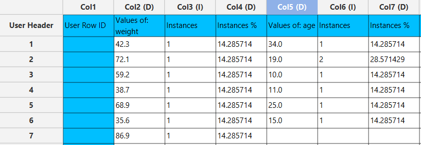
The output displays the frequency and percentage distribution of values for each column in your input dataset. It lists distinct values in each column along with their count (instances) and proportion of the total (% instances), providing a concise summary of the data’s distribution across these variables.
Example
Input
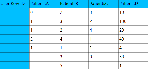
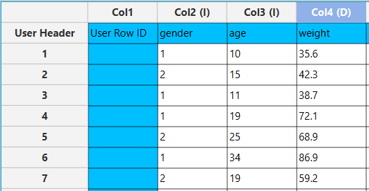
In the left-hand spreadsheet, insert the data for each variable you plan to use for weight cases calculations. In this example, this includes entering the values for gender as integers, age and weight directly into their respective columns. Each row should represent a single data point, ensuring the dataset is structured correctly for further analysis and weight calculation.
Configuration
- Select
Statistics\(\rightarrow\)Basic Statistics\(\rightarrow\)Weight Cases. - Select the columns that are going to be used for weight cases calculation by clicking on the arrow buttons [3] and moving columns between the
Excluded Columns[1] andIncluded Columns[2] lists. In this case the calculations are performed only for the columns 3-“age” and 4-“weight”. - Click on the
Executebutton [4] to apply the weight cases calculation on the selected columns.

Output
In the right-hand spreadsheet of the tab the output data displays the count (instances) and percentage of the total occurrences (instances %) for each unique value for the selected columns.
References
- Jones, J.S., Exploratory and descriptive statistics. 2022: SAGE Publications Limited.
- Smithson, M., Confidence intervals. 2003: Sage. doi.org/10.4135/9781412983761
- Meeker, W.Q., G.J. Hahn, and L.A. Escobar, Statistical intervals: a guide for practitioners and researchers. Vol. 541. 2017: John Wiley & Sons.
- Moore, DS, McCabe, GP. Introduction to the practice of statistics. WH Freeman/Times Books/Henry Holt & Co.; 1989.
- Bluman, A. Elementary Statistics: A step by step approach 9e. McGraw Hill.; 2014.
- Valliant, R. and J.A. Dever, Survey weights: a step-by-step guide to calculation. Vol. 1. 2018: Stata Press College Station, TX.
Version History
Introduced in Isalos Analytics Platform v0.2.4
Instructions last updated on June 2026