








Clustering
Cluster analysis is an unsupervised learning technique that is able to group instances into clusters based on the distinct characteristics of the data points. Unsupervised learning operates on unlabeled data and focuses on learning from input without human supervision. The goal of clustering is to divide unlabeled objects into meaningful groups where items in each subset are similar to each other rather than to instances in other subsets. This method is often used for data exploration, facilitating the identification of underlying patterns within the dataset that are not immediately obvious. 1,2
Table of contents
K-Means
K-Means is a simple non-parametric clustering algorithm used for partitioning samples into separated clusters of equal variance. The algorithm begins by randomly selecting K observation instances as the initial centroids, then proceeds by assigning each observation to the cluster whose centroid is closest to it. Different distance-based methods can be employed to calculate the respective distances between datapoints. The centroids are then recomputed as the average of the observations allocated to the cluster. This process is repeated until the assignment of observations to clusters no longer changes significantly, or after a fixed number of iterations. The K parameter denotes the number of clusters that are formed. 1,2
Use the K-Means clustering function by browsing in the top ribbon:
| Analytics \(\rightarrow\) Clustering \(\rightarrow\) K-Means |
Input
Data matrix with training set data. String columns are not taken into account in the algorithm implementation since K-means does not allow the use of nominal (categorical) input.
Configuration
| Number of centroids | Specify an integer representing the number of centroids (K) to generate, coresponding to the number of clusters that form (default value: 3). |
| Number of iterations | Specify the maximum number of times the algorithm runs to converge with different centroids (default value: 100). |
| Distance method | Select the metric used to calculate distances between data points. Three options are available for selection: - Manhattan/L1: Sum of the absolute differences between coordinates of instances pairs, - Euclidean/L2: Square root of differences between coordinates of instances pairs, and - Cosine: Uses cosine distance to determine how two features are oriented relative to each other, based on the angle between the vectors rather than their magnitude. |
| Initialization | Select the method used for the initialization. Two options are available for selection: - Random: Cluster centroids are randomly selected for initialization, and - KMeans++: Improved cluster initialization technique that uses a heuristic to find centroid seeds. For more information on K-means++ see in Arthur et al.3. |
| Number of threads | Isalos supports multi-threading for K-Means. Specify the number of threads to use for computation (default value: 100). |
| RNG Seed | Select an integer as seed to get reproducible results. The option to select a time-based random number-generated seed is available by clicking on the Time Based RNG Seed checkbox. |
Output
A data matrix listing the characteristics of each centroid and cluster assignment information is presented.
Example
Input
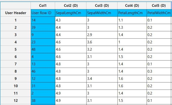
In the left-hand spreadsheet of the tab import the data matrix. In case that categorical features are included in the input data matrix, an error message appears: “K-means does not allow the use of nominal (categorical) input. To proceed please remove column(s)”.
Configuration
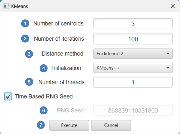
- Select
Analytics\(\rightarrow\)Clustering\(\rightarrow\)K-Means. - Select the
Number of clusters[1], and theNumber of iterations[2] the algorithm will run to converge. - Select the
Distance method[3] that determines the centroid closest to an instance and determine theInitializationmethod [4]. - Select the
Number of threadsto choose the single-threaded or multi-threaded version of the algorithm [5]. - Select an RNG Seed for reproducible results or a random number generated
Time Based RNG Seed[6]. - Click on the
Executebutton [7] to apply the training algorithm on the input columns.
Output
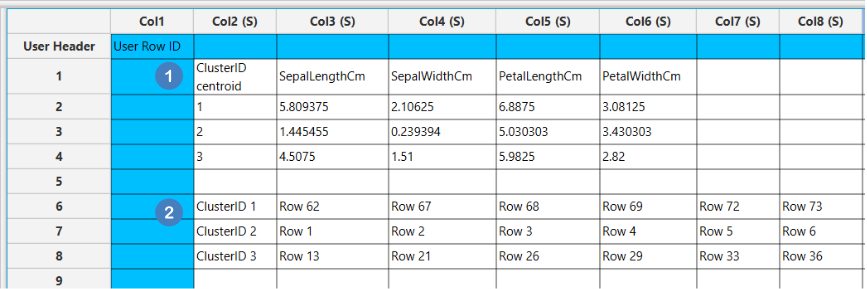
In the right-hand spreadsheet of the tab the output data matrix with the centroid and cluster assignment information is presented. The first section lists the centroids of each cluster with an identifier [1] and presents the average value of the points that are assigned to each respective cluster for all the numerical variables in the dataset. In the second section [2] the data points assigned to each cluster are presented horizontally.
Application on external set
You can apply the trained K-Means model to any external (test) data using the Existing Model Utilization function:
- Import the external data in the left-hand spreadsheet of the tab. Include the same columns used to build the K-Means model.
- Select
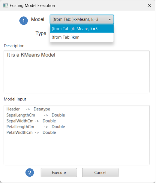
Analytics\(\rightarrow\)Existing Model Utilization. Select the K-Means model [1] and click on theExecutebutton [2].
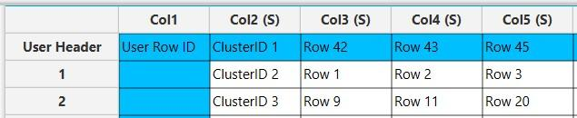
- Inspect the results in the right-hand spreadsheet of the tab.
DBSCAN
DBSCAN is a density-based clustering algorithm that groups together data points that are close to each other based on a specified distance metric, while marking points that lie alone in low-density regions as outliers (noise). Unlike algorithms such as k-means, DBSCAN does not require predefining the number of clusters, making it well-suited for exploratory data analysis where the underlying cluster structure is unknown.
There are are two key parameters in this algorithm:
- Epsilon: This is a numeric value that defines the radius of the neighborhood around a data point. Two point are set to be neighbors if the distance between them is less than eps. Choosing the correct value for this parameter is vital as a small Epsilon will result in a lot of outliers and a large Epsilon will merge clusters together.
- Min Points: This is an integer value that specifies how many points are required in a neighborhood for that to be characterized as dense. A genera rule is to set the Min Points parameter to k + 1 where k is the dimensionality of the feature space.
DBSCAN offers several advantages that make it a powerful and flexible clustering method. It can automatically determine the number of clusters based on the data’s density distribution, eliminating the need for manual input or prior assumptions. The algorithm can identify clusters of arbitrary shape and size, which is especially useful for complex or non-spherical data distributions. Moreover, DBSCAN is robust to outliers and noise, effectively separating them from meaningful cluster structures. It also performs well on datasets with varying cluster densities and does not require feature scaling to a specific range, though normalization can still improve performance.
Use the DBSCAN clustering function by browsing in the top ribbon:
| Analytics \(\rightarrow\) Clustering \(\rightarrow\) DBSCAN |
Input
Data matrix with training set data. Numerical and categorical columns are allowed. Differences in values in categorical columns are treated as 0/1.
Configuration
| Epsilon | Specify a positive double value representing the radius of each neighborhood. Default value is set to 0.5 |
| Min Points | Specify an integer value that represents the minimum number of points that have to be inside an Epsilon neighborhood for that neighborhood to be labeled as dense. |
Output
Cluster assignment information is presented.
Example
Input
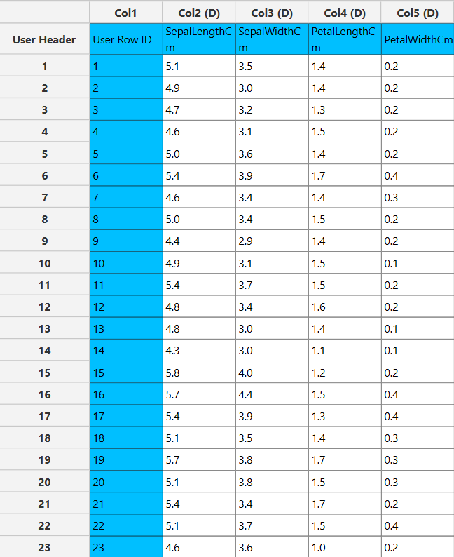
In the left-hand spreadsheet of the tab import the data matrix with the data points that are to be clustered.
Configuration
- Select
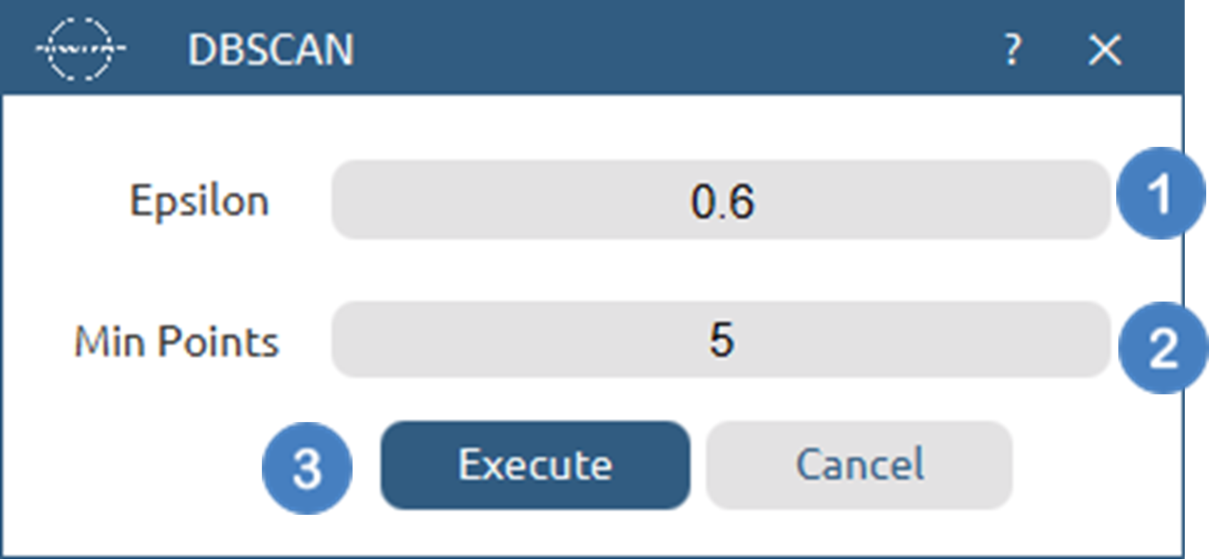
Analytics\(\rightarrow\)Clustering\(\rightarrow\)DBSCAN. - Select the value for
Epsilon[1] - Select the
Minimum Points[2] that should exist in a region for that to be labeled as dense. - Click on the
Executebutton [3] to apply the algorithm on the input columns.
Output
In the right-hand spreadsheet of the tab the output data matrix with the cluster assignment information is presented where data points assigned to each cluster are presented horizontally.

Hierarchical Clustering
Hierarchical Clustering is a clustering algorithm that builds a nested hierarchy of cluster partitions rather than producing a single flat assignment. Two strategies are supported: Agglomerative (bottom-up), which starts with every point as its own cluster and successively merges the closest pair, and Divisive (top-down), which starts with all points in one cluster and recursively splits the largest cluster until the stopping criterion is met. The result is visually a tree-like structure (dendrogram) whose branches can be cut at any level to obtain a desired number of clusters or at a specified distance threshold. 6
Hierarchical clustering does not require the number of clusters to be fixed in advance when the cutoff mode is used, and it provides a complete picture of the data’s cluster structure at all granularities.
Agglomerative (bottom-up)
Each observation starts as its own cluster. At every step the two active clusters with the smallest linkage distance are merged. Distance updates between the newly merged cluster and all remaining clusters are computed using the Lance-Williams recurrence:
\[d(k,\, i \cup j) = \alpha_i \cdot d(k,i) + \alpha_j \cdot d(k,j) + \beta \cdot d(i,j) + \gamma \cdot |d(k,i) - d(k,j)|\]where the coefficients (αi, αj, β, γ) depend on the chosen linkage function:
| Linkage | αi | αj | β | γ |
|---|---|---|---|---|
| Single | 1/2 | 1/2 | 0 | −1/2 |
| Complete | 1/2 | 1/2 | 0 | +1/2 |
| Average | nA/(nA+nB) | nB/(nA+nB) | 0 | 0 |
| Ward / ward.D2 | (nK+nA)/(nK+nA+nB) | (nK+nB)/(nK+nA+nB) | −nK/(nK+nA+nB) | 0 |
| Mcquitty | 1/2 | 1/2 | 0 | 0 |
| Median | 1/2 | 1/2 | −1/4 | 0 |
For Ward and ward.D2 the initial distance matrix stores squared Euclidean distances; the Lance-Williams formula then maintains squared distances throughout.
Divisive (top-down)
All observations start in a single cluster. At every step the largest cluster is selected for splitting: the two most distant points within it are found and used as seeds, and every remaining point in the cluster is assigned to the nearer seed. Splitting continues until the stopping criterion is met.
Stopping criterion
Two modes are available:
- Number of Clusters — merging (agglomerative) or splitting (divisive) stops as soon as the active cluster count reaches the target value.
- Cutoff Value — merging stops when the next merge distance would equal or exceed the threshold; splitting stops when the distance between the two seeds of the next split falls below the threshold.
Distance metrics
| Metric | Formula |
|---|---|
| Euclidean (default) | \(d(a,b) = \sqrt{\sum_k (a_k - b_k)^2}\) |
| Manhattan | \(d(a,b) = \sum_k |a_k - b_k|\) |
| Chebyshev | \(d(a,b) = \max_k |a_k - b_k|\) |
| Cosine | \(d(a,b) = 1 - \dfrac{a \cdot b}{|a|\,|b|}\) |
Use the Hierarchical Clustering function by browsing in the top ribbon:
| Analytics \(\rightarrow\) Clustering \(\rightarrow\) Hierarchical Clustering |
Input
Data matrix with training set data. Only numerical columns are used in the computation; nominal (categorical) columns are not permitted and will produce an error message listing the offending columns.
Configuration
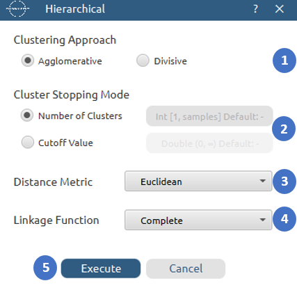
| Clustering Approach | Select the hierarchical strategy: - Agglomerative: bottom-up; starts with each point as its own cluster and merges iteratively. - Divisive: top-down; starts with all points in one cluster and splits iteratively. Default: Agglomerative. |
| Cluster Stopping Mode | Choose how the algorithm decides when to stop: - Number of Clusters: stop when the specified number of clusters is reached. Specify a positive integer. - Cutoff Value: stop when the next merge distance (agglomerative) meets or exceeds the threshold, or the next split distance (divisive) falls below it. Specify a positive value. |
| Distance Metric | Select the metric used to compute pairwise distances between observations. Available options: Euclidean, Manhattan, Chebyshev, Cosine. Default: Euclidean. |
| Linkage Function | Select the criterion used to determine the distance between two clusters during agglomerative merging. Available options: Single, Complete, Average, Ward, Mcquitty, ward.D2, Median. Default: Complete. Note: Ward and ward.D2 linkage require Euclidean distance; the distance metric is automatically set to Euclidean if a non-Euclidean metric is selected alongside Ward or ward.D2. |
Output
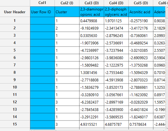
The output table contains a Cluster column (1-based integer label) followed by the original input columns. Each row is assigned to exactly one cluster. Cluster labels are remapped to sequential integers starting from 1 in the order they are first encountered.
Example
Input
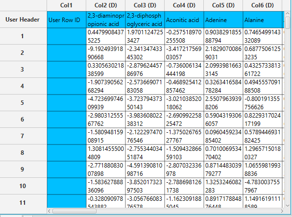
In the left-hand spreadsheet of the tab import the data matrix with the data points that are to be clustered. If any nominal (categorical) columns are present, an error message appears listing the columns that must be removed before execution can proceed.
Configuration
- Select
Analytics\(\rightarrow\)Clustering\(\rightarrow\)Hierarchical Clustering. - Choose the
Clustering Approach[1]: Agglomerative or Divisive. - Select the
Cluster Stopping Mode[2] and enter the corresponding value: a positive integer for Number of Clusters or a positive value for Cutoff Value. - Choose the
Distance Metric[3] to use for computing pairwise distances. - Select the
Linkage Function[4] to use for computing inter-cluster distances (agglomerative only). - Click on the
Executebutton [5] to apply the algorithm on the input columns.
Output
In the right-hand spreadsheet of the tab the output data matrix is presented. The first column contains the cluster assignment for each observation (1-based label), followed by the original input columns.
Tips
- As calculations of Euclidean distances are performed, consider scaling the data beforehand using a
Normalizerfunction. - The K-Means algorithm requires the number of clusters to be specified. Its performance is highly influenced by the initialization of the centroids and the selection of K.
- For Hierarchical Clustering, the choice of linkage function strongly influences the shape and compactness of the resulting clusters. Single linkage tends to produce elongated, chained clusters; Complete linkage produces more compact, evenly sized clusters; Ward linkage minimises within-cluster variance and is generally a robust default for compact clusters.
See also
The model generated by any of the hierarchical clustering algorithms can be applied to any input data through the Existing Model Utilization function (e.g., a K-means model trained from the training set data of a machine learning model can be applied to the test/external set data).
References
- Witten Ian H and Frank, Eibe and Hall, Mark A and Pal CJ. Data Mining: Practical Machine Learning Tools and Techniques. Fourth. Morgan Kaufmann; 2011. https://doi.org/10.1016/C2009-0-19715-5.
- Murphy KP. Machine Learning: A Probabilistic Perspective. The MIT Press; 2012. 10.5555/2380985.
- Arthur, D.; Vassilvitskii, S. K-Means++: The Advantages of Careful Seeding. In Proceedings of the eighteenth annual ACM-SIAM symposium on Discrete algorithms; SODA ’07; Society for Industrial and Applied Mathematics: USA, 2007; pp 1027–1035. 10.5555/1283383.1283494.
- Ester, Martin, Hans-Peter Kriegel, Jörg Sander, and Xiaowei Xu. “A density-based algorithm for discovering clusters in large spatial databases with noise.” In kdd, vol. 96, no. 34, pp. 226-231. 1996. 10.5555/3001460.3001507.
- Schubert, Erich, Jörg Sander, Martin Ester, Hans Peter Kriegel, and Xiaowei Xu. “DBSCAN revisited, revisited: why and how you should (still) use DBSCAN.” ACM Transactions on Database Systems (TODS) 42, no. 3 (2017): 1-21. 10.1145/3068335.
- Murtagh, Fionn, and Pedro Contreras. Algorithms for hierarchical clustering: An overview. Wiley Interdisciplinary Reviews: Data Mining and Knowledge Discovery; 2012; 2(1): 86–97. https://doi.org/10.1002/widm.53.
Version History
Introduced in Isalos Analytics Platform v0.1.18
Instructions last updated on August 2026