Optimal Designs

The theory of optimal designs centers around the problems of characterization and construction of designs which are optimal in some sense from a number of alternative experiments in a given design set-up. The objective in these methods is to choose n points to include in the design from a finite set of N candidate points so that the resulting is optimal in some sense. Different criteria reflect different experimental goals—for example, minimizing the average variance of parameter estimates (A-optimality), maximizing the determinant of the information matrix (D-optimality), maximizing the smallest eigenvalue (E-optimality), or minimizing the worst prediction variance over the candidate set (G-optimality). The choice of criterion guides how designs are evaluated.

To construct optimal (or near-optimal) designs we use the modified Fedorov point-exchange algorithm (Cook & Nachtsheim, 1980). Starting from an initial design of randomly selected candidate points, the algorithm iteratively seeks swaps—replacing one design point with a candidate not in the design—that improve the objective (e.g., D, A, E, or G). Swaps are accepted greedily, and the process continues until no improving exchange exists, at which point the algorithm has converged to a locally optimal design. Multiple trials can be done to hedge against local optima and further improve the final result.

D-Optimal Design

D-Optimal designs are a subcategory of Optimal Designs where the criterion based on which we compare designs focuses on the minimization of the generalized variance of the estimated regression coefficients. Equivalently, they maximize the determinant of the information matrix $M=X^{'}X$ (Where $X$ is the design matrix of the multiple linear regression). Thus, for a design of size q, the objective for our algorithm is:

$$ \begin{equation} max_{d_q} (|X^{'}X|) \end{equation} $$

taken over all feasible designs with q runs. Maximizing $|X^{'}X|$ is the same as minimizing the volume of the joint confidence ellipsoid for the parameters, and in practice we maximize $log|X^{'}X|$ for numerical stability.

Use the D-Optimal Design Function by browsing in the top ribbon:

DOE $\rightarrow$ Optimal Desings $\rightarrow$ D-Optimal Design

Input

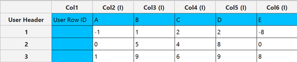
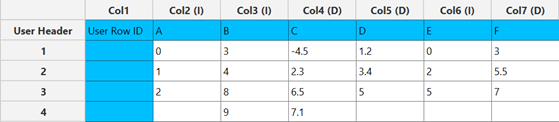
All variables must be specified in the datasheet. The input to the algorithm consists of the factors included in the experiment and their respective levels. Factors can have different numbers of levels, but all entries must be numeric. The function requires at least two factor columns in the spreadsheet.

Configuration

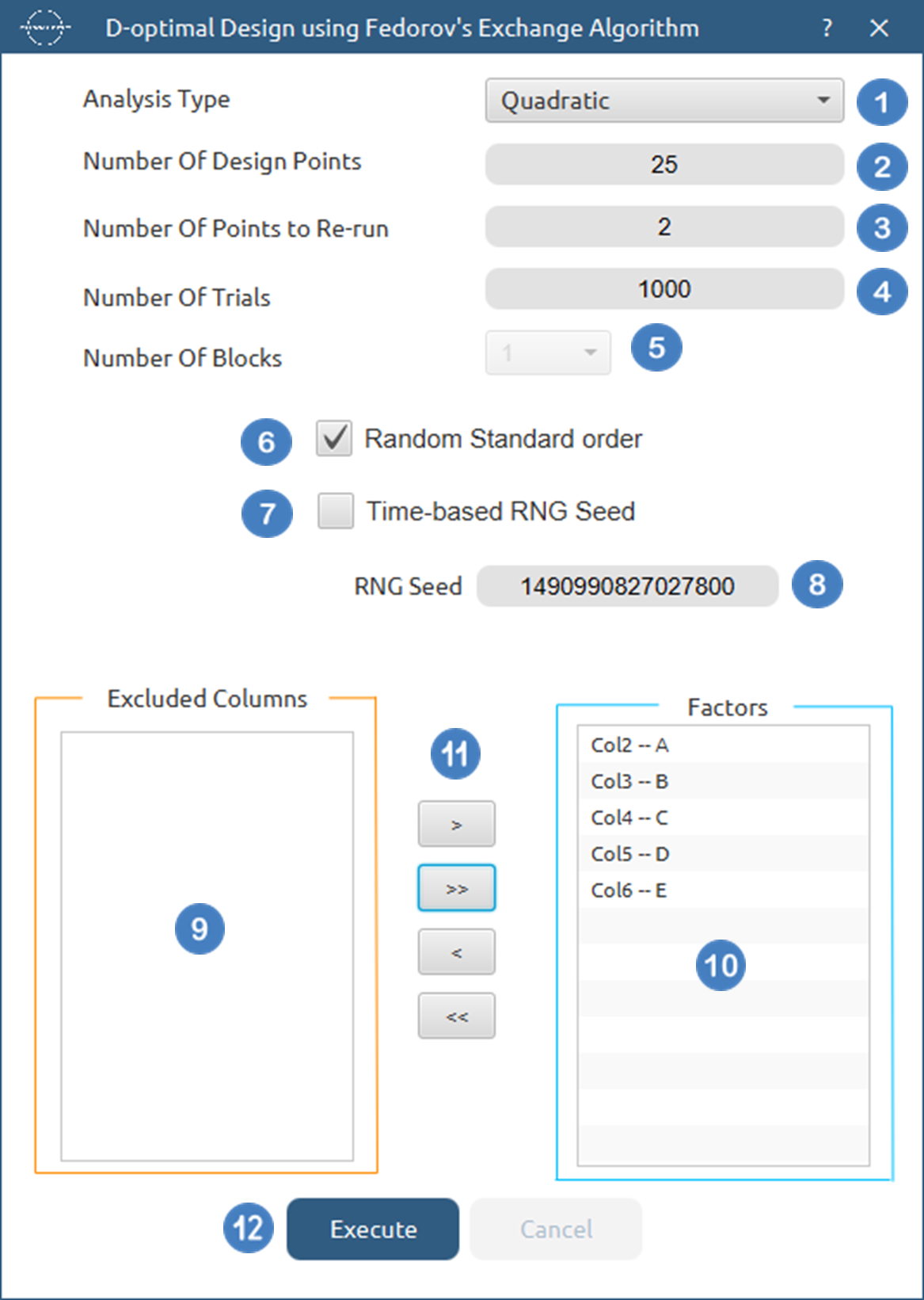
Analysis Type	Select the desired analysis type for the analysis. Available options include: Main Effects, Main Effects + Two-way Interactions, Quadratic. If at least two factors have less than three levels then the quadratic terms cannot be included.
Number of Design Points	Select manually the number of design points to produce. This number should be larger than the number of regression parameters included in the model and smaller than the number of all possible combinations between factor levels. The lower bound for each case of the analysis type for k factors is: Main Effects : $k + 1$, Main Effects and Two-way Interactions : $k + k(k-1)/2 + 1$, Quadratic: $2k + k*(k-1)/2+1$
Number of Points to Re-run	Select manually the number of replicate runs to add. These are exact duplicates of points already in the design (randomly chosen) and are used to provide extra degrees of freedom for pure error and lack-of-fit checks in the regression that follows. Default value is set to 0.
Number of Trials	Select manually the number of times to restart the algorithm from a different random initial solution. More trials reduce the chance of getting stuck in a local optimum and typically yield a more robust design. Default value is set to 1000.
Number of Blocks	Select from the list of available options the `Number of Blocks`. Currently, the only supported option is 1.
Random Standard order	You can tick/select the box if you want to shuffle the order of points randomly.
Time-based RNG Seed	Regardless of if the randomness is selected, a random seed is needed to create the initial conditions of each trial. You have the option to also tick/select the box to set the random generated number seed based on time.
RNG Seed	Select manually the random generated number seed if required.
Factors/Excluded Columns	Select manually the columns that correspond to factors through the dialog window: Use the buttons to move columns between the Factors list and Excluded Columns list. Single-arrow buttons will move all selected columns and double-arrow buttons will move all columns. At least two factor columns should be specified.

Output

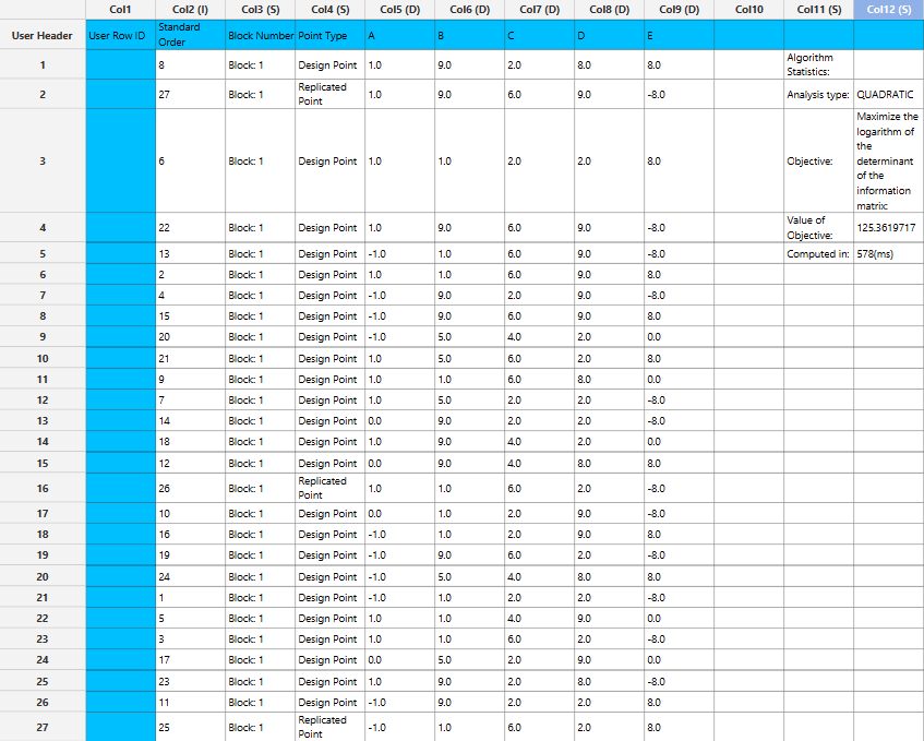
The output consists of two sections:

Design table: The points included in the optimal design calculated. Each row is labeled as Design Point (a unique point chosen from the candidate set) or Replicate (an exact repeat of a previously listed design point) and includes the Standard Order and the Block Number of each data point.
Algorithm Statistics table: A compact summary of the optimization, providing the analysis type selected, the design size , the objective value and the time it took to compute the design (in milliseconds).

Example

Input

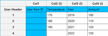
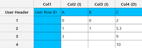
The input datasheet must include at least two numeric factor variables.

Configuration

Select DOE $\rightarrow$ Optimal Desings $\rightarrow$ D-Optimal Desing.
Select the Analysis Type.[1].
Specify the Number of Design Points [2] to produce.
Specify the Number of Replicate Points [3] to produce.
Specify the Number of Trials [4] to perform.
Select the Number of Blocks [5].
Select/tick if required the Random Standard order [6] to imply randomness in order of experiments.
Either select/tick to generate the number seed for randomness based on time [7] or by manually setting a value [8].
Select the columns by clicking on the arrow buttons [11] and moving columns between the Excluded Columns [9] and Factors [10] lists.
Click on the Execute button [12] to compute the D-Optimal Design.

Output

The computed design along with the algorithm statistics will be shown in the output spreadsheet.

A-Optimal Design

A-Optimal designs are a subcategory of Optimal Designs where the criterion based on which we compare designs focuses on the minimization of the average variance of the estimated regression coefficients. Equivalently, they minimize the trace (the sum of diagonal elements) of the inverse of the information matrix $M=X^{'}X$ (Where $X$ is the design matrix of the multiple linear regression). Thus, for a design of size q, the objective for our algorithm is:

$$ \begin{equation} min_{d_q} (trace (X^{'}X)^{-1}) \end{equation} $$

taken over all feasible designs with q runs. A-optimal designs are not invariant to changes in the scaling or the coding of factors unlike D-optimal designs.

Use the A-Optimal Design Function by browsing in the top ribbon:

DOE $\rightarrow$ Optimal Desings $\rightarrow$ A-Optimal Design

Input

Configuration

Analysis Type	Select the desired analysis type for the analysis. Available options include: Main Effects, Main Effects + Two-way Interactions, Quadratic. If at least two factors have less than three levels then the quadratic terms cannot be included.
Number of Design Points	Select manually the number of design points to produce. This number should be larger than the number of regression parameters included in the model and smaller than the number of all possible combinations between factor levels. The lower bound for each case of the analysis type for k factors is: Main Effects : $k + 1$, Main Effects and Two-way Interactions : $k + k(k-1)/2 + 1$, Quadratic: $2k + k*(k-1)/2+1$
Number of Points to Re-run	Select manually the number of replicate runs to add. These are exact duplicates of points already in the design (randomly chosen) and are used to provide extra degrees of freedom for pure error and lack-of-fit checks in the regression that follows. Default value is set to 0.
Number of Trials	Select manually the number of times to restart the algorithm from a different random initial solution. More trials reduce the chance of getting stuck in a local optimum and typically yield a more robust design. Default value is set to 1000.
Number of Blocks	Select from the list of available options the `Number of Blocks`. Currently, the only supported option is 1.
Random Standard order	You can tick/select the box if you want to shuffle the order of points randomly.
Time-based RNG Seed	Regardless of if the randomness is selected, a random seed is needed to create the initial conditions of each trial. You have the option to also tick/select the box to set the random generated number seed based on time.
RNG Seed	Select manually the random generated number seed if required.
Factors/Excluded Columns	Select manually the columns that correspond to factors through the dialog window: Use the buttons to move columns between the Factors list and Excluded Columns list. Single-arrow buttons will move all selected columns and double-arrow buttons will move all columns. At least two factor columns should be specified.

Output

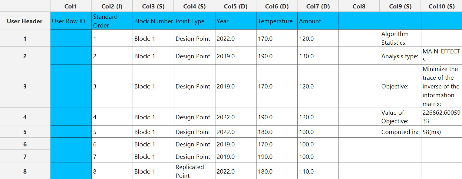
The output consists of two sections:

Design table: The points included in the optimal design calculated. Each row is labeled as Design Point (a unique point chosen from the candidate set) or Replicate (an exact repeat of a previously listed design point) and includes the Standard Order and the Block Number of each data point.
Algorithm Statistics table: A compact summary of the optimization, providing the analysis type selected, the design size , the objective value and the time it took to compute the design (in milliseconds).

Example

Input

The input datasheet must include at least two numeric factor variables.

Configuration

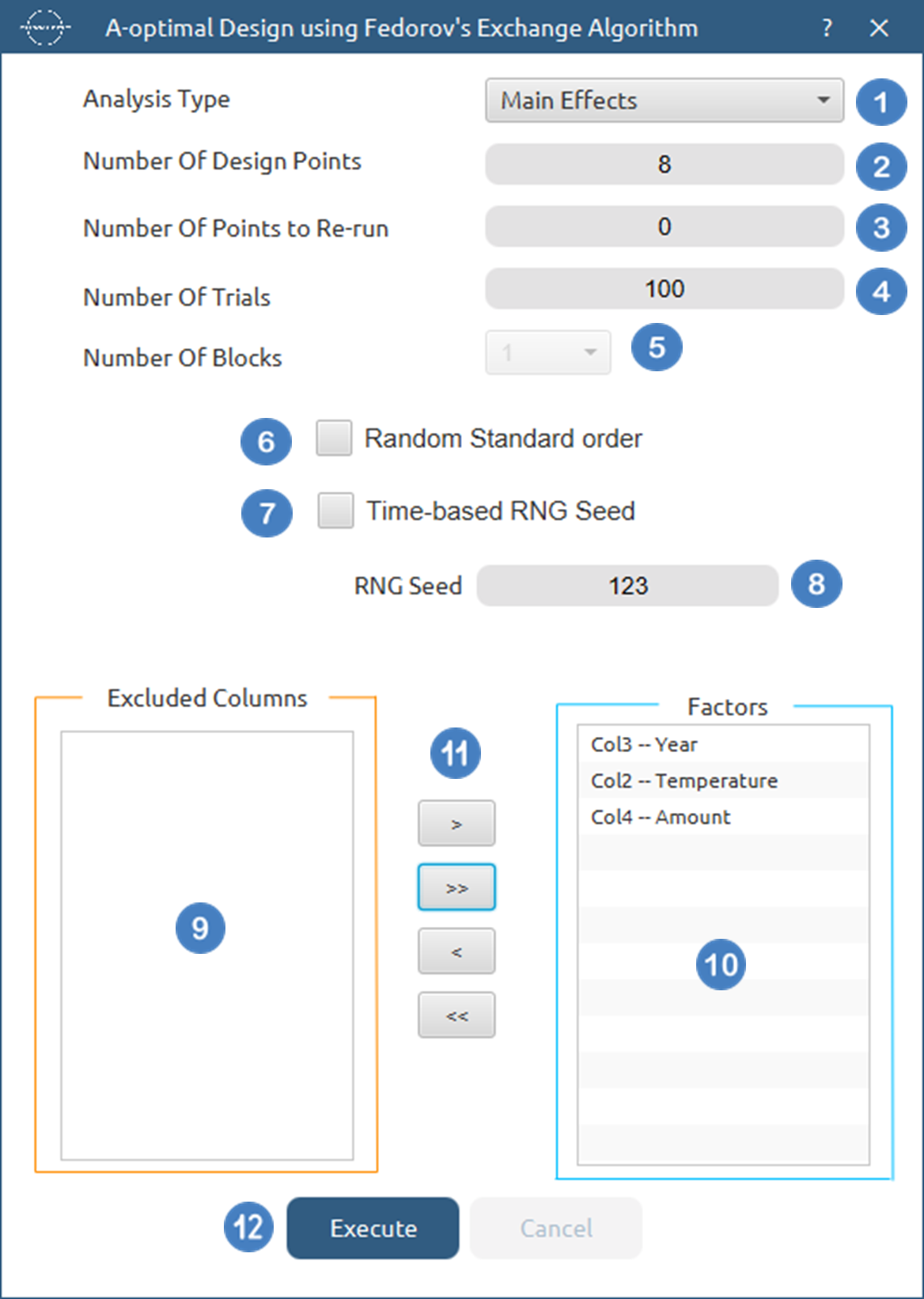
Select DOE $\rightarrow$ Optimal Desings $\rightarrow$ A-Optimal Desing.
Select the Analysis Type.[1].
Specify the Number of Design Points [2] to produce.
Specify the Number of Replicate Points [3] to produce.
Specify the Number of Trials [4] to perform.
Select the Number of Blocks [5].
Select/tick if required the Random Standard order [6] to imply randomness in order of experiments.
Either select/tick to generate the number seed for randomness based on time [7] or by manually setting a value [8].
Select the columns by clicking on the arrow buttons [11] and moving columns between the Excluded Columns [9] and Factors [10] lists.
Click on the Execute button [12] to compute the A-Optimal Design.

Output

The computed design along with the algorithm statistics will be shown in the output spreadsheet.

E-Optimal Design

E-Optimal designs are a class of optimal designs in which the comparison criterion aims to maximize the smallest eigenvalue of the information matrix $M=X^{'}X$ (Where $X$ is the design matrix of the multiple linear regression). Equivalently, this minimizes the largest eigenvalue of $M^{-1}$, controlling the worst-case variance direction. Thus, for a design of size q, the objective is

$$ \begin{equation} max_{d_q} (\lambda \_ min (X^{'}X)) \end{equation} $$

taken over all feasible designs with qruns. Maximizing $\lambda \_ min (X^{'}X)$ tightens the longest axis of the joint confidence ellipsoid for the parameters (i.e., improves the least well-identified direction).

Use the E-Optimal Design Function by browsing in the top ribbon:

DOE $\rightarrow$ Optimal Desings $\rightarrow$ E-Optimal Design

Input

Configuration

Analysis Type	Select the desired analysis type for the analysis. Available options include: Main Effects, Main Effects + Two-way Interactions, Quadratic. If at least two factors have less than three levels then the quadratic terms cannot be included.
Number of Design Points	Select manually the number of design points to produce. This number should be larger than the number of regression parameters included in the model and smaller than the number of all possible combinations between factor levels. The lower bound for each case of the analysis type for k factors is: Main Effects : $k + 1$, Main Effects and Two-way Interactions : $k + k(k-1)/2 + 1$, Quadratic: $2k + k*(k-1)/2+1$
Number of Points to Re-run	Select manually the number of replicate runs to add. These are exact duplicates of points already in the design (randomly chosen) and are used to provide extra degrees of freedom for pure error and lack-of-fit checks in the regression that follows. Default value is set to 0.
Number of Trials	Select manually the number of times to restart the algorithm from a different random initial solution. More trials reduce the chance of getting stuck in a local optimum and typically yield a more robust design. Default value is set to 1000.
Number of Blocks	Select from the list of available options the `Number of Blocks`. Currently, the only supported option is 1.
Random Standard order	You can tick/select the box if you want to shuffle the order of points randomly.
Time-based RNG Seed	Regardless of if the randomness is selected, a random seed is needed to create the initial conditions of each trial. You have the option to also tick/select the box to set the random generated number seed based on time.
RNG Seed	Select manually the random generated number seed if required.
Factors/Excluded Columns	Select manually the columns that correspond to factors through the dialog window: Use the buttons to move columns between the Factors list and Excluded Columns list. Single-arrow buttons will move all selected columns and double-arrow buttons will move all columns. At least two factor columns should be specified.

Output

The output consists of two sections:

Design table: The points included in the optimal design calculated. Each row is labeled as Design Point (a unique point chosen from the candidate set) or Replicate (an exact repeat of a previously listed design point) and includes the Standard Order and the Block Number of each data point.
Algorithm Statistics table: A compact summary of the optimization, providing the analysis type selected, the design size , the objective value and the time it took to compute the design (in milliseconds).

Example

Input

The input datasheet must include at least two numeric factor variables.

Configuration

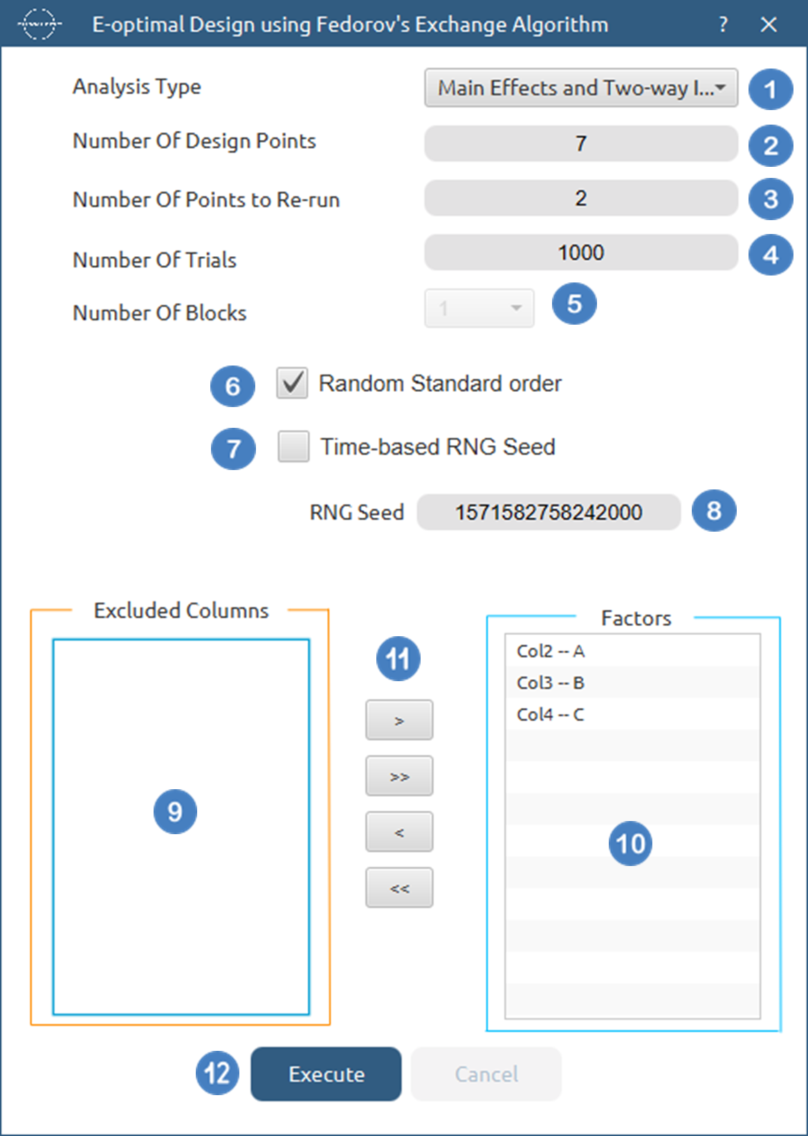
Select the Analysis Type.[1].
Specify the Number of Design Points [2] to produce.
Specify the Number of Replicate Points [3] to produce.
Specify the Number of Trials [4] to perform.
Select the Number of Blocks [5].
Select/tick if required the Random Standard order [6] to imply randomness in order of experiments.
Either select/tick to generate the number seed for randomness based on time [7] or by manually setting a value [8].
Select the columns by clicking on the arrow buttons [11] and moving columns between the Excluded Columns [9] and Factors [10] lists.
Click on the Execute button [12] to compute the E-Optimal Design.

Output

The computed design along with the algorithm statistics will be shown in the output spreadsheet.

G-Optimal Design

G-optimal designs are a class of optimal designs in which the comparison criterion aims to minimize the worst-case prediction variance over a specified candidate (or design) space. For a linear model with information matrix $M=X^{'}X$ and regressor vector $c(x)$ at point $x$, the scaled prediction variance at $x$ is $c(x)^{'} M^{-1} c(x)$. Thus, for a design of size q, the objective is:

$$ \begin{equation} min_{d_q} (max_{x \in \mathcal{C}} (c(x) ^{'} (X^{'}X)^{-1} c(x))) \end{equation} $$

taken over all feasible designs with qruns and candidate set $\mathcal{C}$. Minimizing this maximum controls the largest prediction uncertainty anywhere in the region. (By the Kiefer–Wolfowitz equivalence theorem, D-optimal designs also minimize this quantity, so D- and G-criteria are closely linked.)

Use the G-Optimal Design Function by browsing in the top ribbon:

DOE $\rightarrow$ Optimal Desings $\rightarrow$ G-Optimal Design

Input

Configuration

Analysis Type	Select the desired analysis type for the analysis. Available options include: Main Effects, Main Effects + Two-way Interactions, Quadratic. If at least two factors have less than three levels then the quadratic terms cannot be included.
Number of Design Points	Select manually the number of design points to produce. This number should be larger than the number of regression parameters included in the model and smaller than the number of all possible combinations between factor levels. The lower bound for each case of the analysis type for k factors is: Main Effects : $k + 1$, Main Effects and Two-way Interactions : $k + k(k-1)/2 + 1$, Quadratic: $2k + k*(k-1)/2+1$
Number of Points to Re-run	Select manually the number of replicate runs to add. These are exact duplicates of points already in the design (randomly chosen) and are used to provide extra degrees of freedom for pure error and lack-of-fit checks in the regression that follows. Default value is set to 0.
Number of Trials	Select manually the number of times to restart the algorithm from a different random initial solution. More trials reduce the chance of getting stuck in a local optimum and typically yield a more robust design. Default value is set to 1000.
Number of Blocks	Select from the list of available options the `Number of Blocks`. Currently, the only supported option is 1.
Random Standard order	You can tick/select the box if you want to shuffle the order of points randomly.
Time-based RNG Seed	Regardless of if the randomness is selected, a random seed is needed to create the initial conditions of each trial. You have the option to also tick/select the box to set the random generated number seed based on time.
RNG Seed	Select manually the random generated number seed if required.
Factors/Excluded Columns	Select manually the columns that correspond to factors through the dialog window: Use the buttons to move columns between the Factors list and Excluded Columns list. Single-arrow buttons will move all selected columns and double-arrow buttons will move all columns. At least two factor columns should be specified.

Output

The output consists of two sections:

Design table: The points included in the optimal design calculated. Each row is labeled as Design Point (a unique point chosen from the candidate set) or Replicate (an exact repeat of a previously listed design point) and includes the Standard Order and the Block Number of each data point.
Algorithm Statistics table: A compact summary of the optimization, providing the analysis type selected, the design size , the objective value and the time it took to compute the design (in milliseconds).

Example

Input

The input datasheet must include at least two numeric factor variables.

Configuration

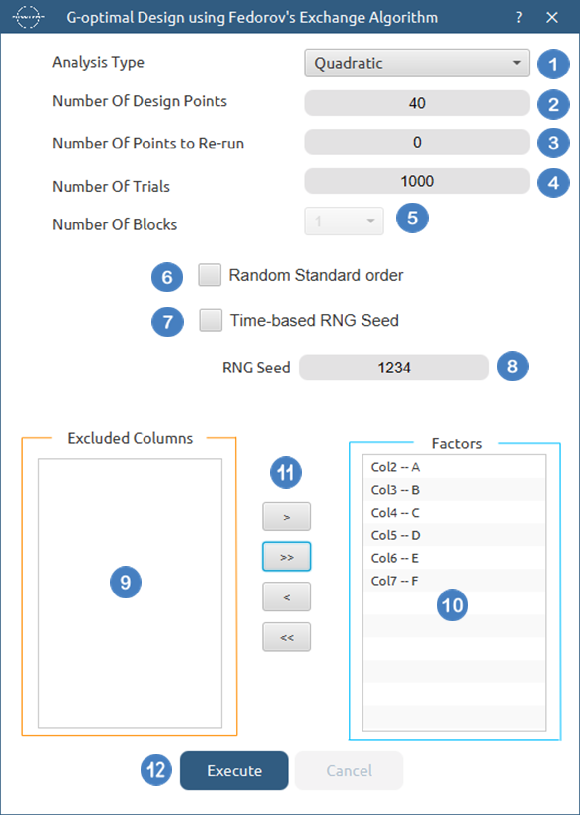
Select DOE $\rightarrow$ Optimal Desings $\rightarrow$ G-Optimal Desing.
Select the Analysis Type.[1].
Specify the Number of Design Points [2] to produce.
Specify the Number of Replicate Points [3] to produce.
Specify the Number of Trials [4] to perform.
Select the Number of Blocks [5].
Select/tick if required the Random Standard order [6] to imply randomness in order of experiments.
Either select/tick to generate the number seed for randomness based on time [7] or by manually setting a value [8].
Select the columns by clicking on the arrow buttons [11] and moving columns between the Excluded Columns [9] and Factors [10] lists.
Click on the Execute button [12] to compute the G-Optimal Design.

Output

The computed design along with the algorithm statistics will be shown in the output spreadsheet.

References

Nguyen, N.K. and Miller, A.J., 1992. A review of some exchange algorithms for constructing discrete D-optimal designs. Computational Statistics & Data Analysis, 14(4), pp.489-498. doi.org/10.1016/0167-9473(92)90064-M.
Gentleman, W.M., 1974. Algorithm AS 75: Basic procedures for large, sparse or weighted linear least problems. Journal of the Royal Statistical Society. Series C (Applied Statistics), 23(3), pp.448-454. doi.org/10.2307/2347147.
Shah, K.R. and Sinha, B.K., 2008. Lecture Notes for Statistics.
Jones, B., Allen-Moyer, K. and Goos, P., 2021. A-optimal versus D-optimal design of screening experiments. Journal of Quality Technology, 53(4), pp.369-382. doi.org/10.1080/00224065.2020.1757391.
Pukelsheim, F., 2007. Optimum Experimental Designs, with SAS by Anthony Atkinson, Alexander Donev, Randall Tobias.

Version History

Introduced in Isalos Analytics Platform v0.2.4

Instructions last updated on November 2025