Analysis of (Co)Variance
The Analysis of (Co)Variance section includes a range of statistical methods designed to test differences in means across groups, while optionally accounting for multiple variables or repeated measures. These techniques are extensions of ANOVA (Analysis of Variance) and ANCOVA (Analysis of Covariance), and they are essential tools in experimental design and multivariate analysis. Many methods are provided, from more simple and straightforward ones, e.g. One-Way ANOVA to more complex ones, allowing for covariances (ANCOVA), repeated measures (Repeated Measures ANOVA) and mixed effects (Mixed ANOVA).
One-Way ANOVA
This is the most basic form of ANOVA and is used when there is only one independent variable with more than two levels or groups. It assesses whether there are any statistically significant differences among the means of the groups. This means that there are two hypotheses: the null hypothesis (H₀) states that all group means are equal, while the alternative hypothesis (H₁) states that at least one of the means is different. To test these hypotheses, One-Way ANOVA calculates two types of variability: the variability between the group means, and the variability within each group. These are used to compute the F-statistic, which measures how much the group means differ relative to the variation inside the groups. A large F-value suggests that the differences between group means are more than what would be expected by chance. Based on this F-value, a p-value is derived. If the p-value is smaller than the chosen significance level (usually 0.05), the null hypothesis is rejected, indicating that not all group means are equal. They are computed using the following equations:
- Sum of Squares $$ \begin{equation} SS_{total} = \sum_{i=1}^N (X_i - \bar{X})^2 {\qquad [1] \qquad} \end{equation} $$
Where \(\bar{X} = \frac{1}{N}\sum_{i=1}^NX_i\), N is the total number of observations from all groups.
$$ \begin{equation} SS_{between} = \sum_{j=1}^N n_j(\bar{X_j} - \bar{X})^2 {\qquad [2] \qquad} \end{equation} $$Where \(\bar{X_j}\) is the mean of group j, \(n_j\) is the number of observations in group j and k is the number of groups
$$ \begin{equation} SS_{within} = SS_{total}-SS_{between} {\qquad [3] \qquad} \end{equation} $$ - F-statistic $$ \begin{equation} F = \frac{SS_{between}/(k-1)}{SS_{within}/(N-k)} {\qquad [4] \qquad} \end{equation} $$
Where k-1 are the degrees of freedom between the groups and N-k are the degrees of freedom within the groups
Use One-Way ANOVA by browsing in the top ribbon:
| Statistics \(\rightarrow\) Analysis of (Co)Variance \(\rightarrow\) One-Way ANOVA |
Input
Numerical values should be specified in the input datasheet. The design for One-Way ANOVA requires at least two columns in the input sheet: one column representing the categorical factor (independent variable), and another column for the numerical response variable (dependent variable). The factor column should contain group labels, and the response column should contain the corresponding measurements for each observation. Each row represents a single observation.
Configuration
| Factor | Select manually the column that corresponds to the factor. |
| Response Variable | Select the column that corresponds to values of the dependent variable. |
Output
The output includes a table summarizing the analysis of variance/covariance. More specifically:
- Sum of Squares (SS): The variation attributed to the term.
- Degrees of Freedom (DF): The number of degrees of freedom associated with the term.
- Mean Square (MS): The sum of squares divided by the degrees of freedom for the term.
- F-statistic: The ratio of the mean square of the term to the mean square of the residuals, used to test the statistical significance of the term.
- p-value: The probability of observing an F-statistic as extreme as the one calculated, assuming the null hypothesis is true.
Example
Input
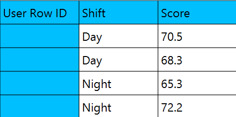
In the input datasheet minimum requirement is to specify one factor (columns) and insert minimum two levels (values) for each factor (column) and one dependent variable with numeric values, as shown below.
Configuration
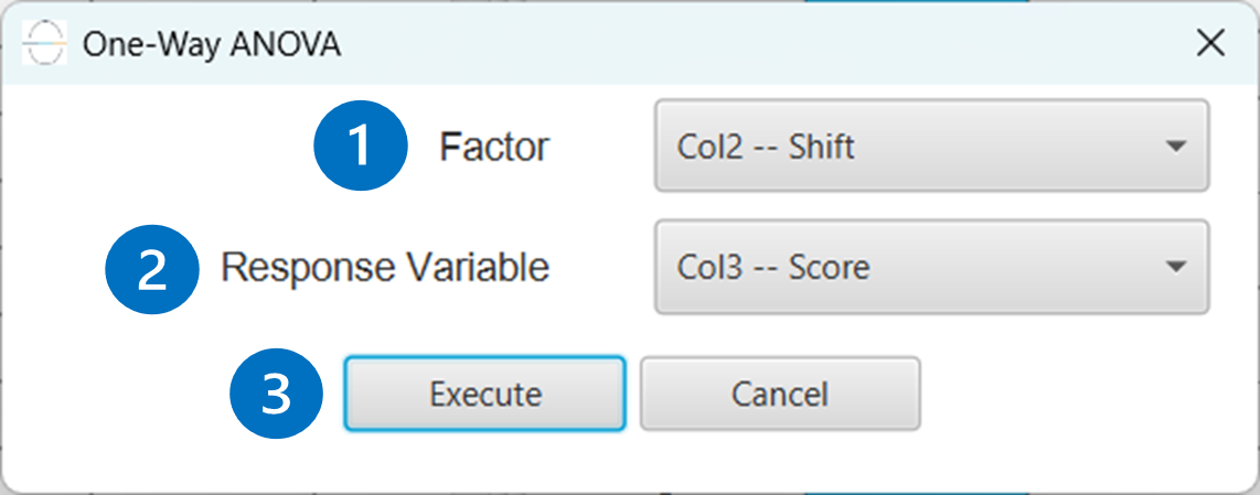
- Select
Statistics\(\rightarrow\)Analysis of (Co)Variance\(\rightarrow\)One-Way ANOVA. - Select the column that correspond to the
Factor[1]. - Select the column that correspond to the
Response Variable[2]. - Click on the
Executebutton [3] to perform the One-Way ANOVA method.
Output
The statistical table of the analysis will be shown in the output spreadsheet.

Two-Way ANOVA
Two-Way ANOVA (Analysis of Variance) is a statistical technique used to examine the effects of two independent categorical variables (called factors) on a single continuous dependent variable. Unlike One-Way ANOVA, which analyzes the effect of only one factor, Two-Way ANOVA allows researchers to evaluate both main effects (the individual impact of each factor) and the interaction effect between the two factors. An interaction occurs when the effect of one factor on the dependent variable changes depending on the level of the other factor. This can reveal complex relationships that would be missed in simpler analyses. This method is particularly useful in experimental designs where you want to study how two different conditions or treatments influence an outcome, both independently and in combination. In a Two-Way ANOVA, three sets of hypotheses are tested:
- The null hypothesis for Factor A assumes that all group means across levels of Factor A are equal (i.e., Factor A has no effect),1. The null hypothesis for Factor B assumes the same for Factor B,
- The null hypothesis for the interaction assumes that there is no interaction effect between the two factors (i.e., the effect of one factor does not depend on the level of the other). If the corresponding p-values are below the chosen significance level (e.g., 0.05), we reject the null hypothesis, indicating that the factor (or interaction) has a statistically significant effect on the dependent variable.
Use Two-Way ANOVA by browsing in the top ribbon:
| Statistics \(\rightarrow\) Analysis of (Co)Variance \(\rightarrow\) Two-Way ANOVA |
Input
Numerical values should be specified in the input datasheet. The design for Two-Way ANOVA requires at least three columns in the input sheet: two columns representing the categorical factors (independent variables) and one column for the numerical response variable (dependent variable). Each row should represent a single observation, with values indicating the level of Factor A, the level of Factor B, and the corresponding measurement of the response variable. The data should be structured so that all combinations of factor levels can be analyzed, as the interaction effect between the two factors is automatically included in the analysis and requires the presence of all level combinations to be estimated properly.
Configuration
| Factor A | Select manually the column that corresponds to the first factor |
| Factor B | Select manually the column that corresponds to the second factor |
| Response Variable | Select the column that corresponds to values of the dependent variable. |
Output
The output includes a table summarizing the analysis of variance/covariance. For each term, including factors and interaction terms, the following information is provided:
- Source: The name of the factor or interaction term.
- Degrees of Freedom (DF): The number of degrees of freedom associated with the term.
- Sum of Squares (SS): The variation attributed to the term.
- Mean Square (MS): The sum of squares divided by the degrees of freedom for the term.
- F-value: The ratio of the mean square of the term to the mean square of the residuals, used to test the statistical significance of the term.
- p-value: The probability of observing an F-statistic as extreme as the one calculated, assuming the null hypothesis is true.
Example
Input
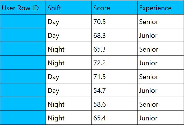
In the input datasheet minimum requirement is to specify two factor (columns) and insert minimum two levels (values) for each factor (column) (All combinations of the levels of factors should appear at least once) and one dependent variable with numeric values, as shown below.
Configuration
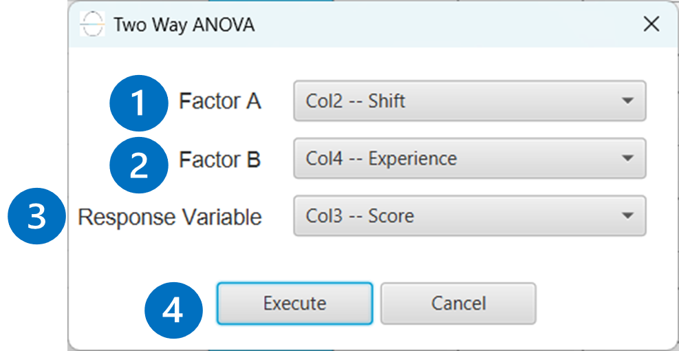
- Select
Statistics\(\rightarrow\)Analysis of (Co)Variance\(\rightarrow\)Two-Way ANOVA. - Select the column that correspond to the
Factor A[1]. - Select the column that correspond to the
Factor B[2]. - Select the column that correspond to the
Response Variable[3]. - Click on the
Executebutton [4] to perform the Two-Way ANOVA method.
Output
The statistical table of the analysis will be shown in the output spreadsheet.
Factorial ANOVA
Factorial ANOVA (Factorial Analysis of Variance) is an extension of the traditional ANOVA method that allows researchers to examine the effects of two or more independent categorical variables—called factors—on a single continuous dependent variable. While One-Way ANOVA tests for differences between groups based on a single factor, Factorial ANOVA moves a step further by considering multiple factors simultaneously. This makes it possible to not only assess the main effects of each individual factor but also to explore interaction effects, that is, whether the effect of one factor depends on the level of another. This approach divides the sample into groups based on all possible combinations of factor levels, allowing for a more detailed and nuanced analysis. However, the user is also given the option to choose whether to include all possible combinations or to analyze only a selected subset of them, depending on the research objectives or experimental constraints. Some researchers also use Factorial ANOVA to explore cause-and-effect relationships. When independent variables represent experimental treatments or controlled conditions, the analysis can help determine whether these manipulations lead to statistically significant changes in the outcome. By organizing observations into groups according to combinations of factor levels, the method compares group means and provides F-tests to assess whether observed differences are likely due to experimental factors rather than chance. Factorial ANOVA is especially powerful in experimental designs, as it mirrors real-world situations where multiple variables often influence outcomes together. When only two factors are involved, the method is typically referred to as Two-Way ANOVA. With three or more factors, it is often called N-Way or general Factorial ANOVA.
Use Factorial ANOVA by browsing in the top ribbon:
| Statistics \(\rightarrow\) Analysis of (Co)Variance \(\rightarrow\) Factorial ANOVA |
Input
Numerical values should be specified in the input datasheet. The design for Factorial ANOVA requires at least two categorical columns to be used as factors (independent variables) and one numerical column as the dependent variable. Each row must represent a single observation, with the factor columns indicating the group levels, and the response column containing the corresponding measurement. The data should be organized so that all combinations of factor levels can be analyzed. This is especially important when the interaction terms are included in the model, as proper estimation of interactions depends on having sufficient representation for each combination of factor levels.
Configuration
| Confidence Level (%) | Specify the confidence level of the analysis. Values should range from 0 to 100 and correspond to percentages. |
| Dependent Variable | Select the column that corresponds to values of the dependent variable. |
| Sum of Squares for Tests | Select method for calculating the significance of factors, covariates and interactions from the two options provided : Adjusted (Type III), Sequential (Type I). When Sequential (Type I) SS is selected be cautious as the order of terms affects the results of the method. When Include Main Effects or Full Factorial formula options are selected, terms are added in the same order as they appear in the configuration window. If you need a specific order, please use the ‘Custom’ formula option. |
| Coding for Factors | Select the type of coding used to code categorical factors from the two options provided: (-1,0,+1), (1,0) |
| Factors/ Exclude Columns | Select manually the columns that correspond to factors through the dialog window. Use the buttons to move columns between the “Excluded Columns” list and the “Factors” list. Single-arrow buttons will move only the selected columns, while double-arrow buttons will move all available columns. At least two categorical columns should be selected as factors, along with one numerical dependent variable. |
| Specify Reference Levels | If the (1,0) coding is selected, specify the reference level for each of the categorical factors specified. The default option for each factor is its last level. |
| Formula Type | These options refer to the terms that will be included in the model. The Custom option allows the user to input a formula defining the exact terms to be included. The Main Effects option allows the analysis of a model that only includes all main effects and finally, the Full Factorial option includes both all main effects and all possible interaction terms to build a full model. |
| Specify Custom Model Formula | Specify the model formula used for the analysis if the Custom option is selected. The formula is created in the Custom Formula Creation dialog window by selecting factors and covariates and adding interaction terms up to the required order. Main effects of the included columns are always part of the model and cannot be excluded. |
Output
The output includes a table summarizing the analysis of variance/covariance. For each term specified in the model formula — including factors and interaction terms — the following information is provided:
- Source: The name of the factor or interaction term.
- Degrees of Freedom (DF): The number of degrees of freedom associated with the term.
- Sum of Squares (SS): The variation attributed to the term, either adjusted (Type III) or sequential (Type I), depending on the method used.
- Mean Square (MS): The sum of squares divided by the degrees of freedom for the term.
- F-statistic: The ratio of the mean square of the term to the mean square of the residuals, used to test the statistical significance of the term.
- P-value: The probability of observing an F-statistic as extreme as the one calculated, assuming the null hypothesis is true.
- Significant: A binary column specifying whether the term is significant based on the specified confidence level and the calculated P-value.
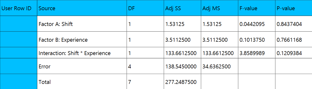
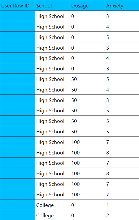
Example
Input
In the input datasheet the requirement is to specify at least two columns and insert the appropriate data, as shown below.
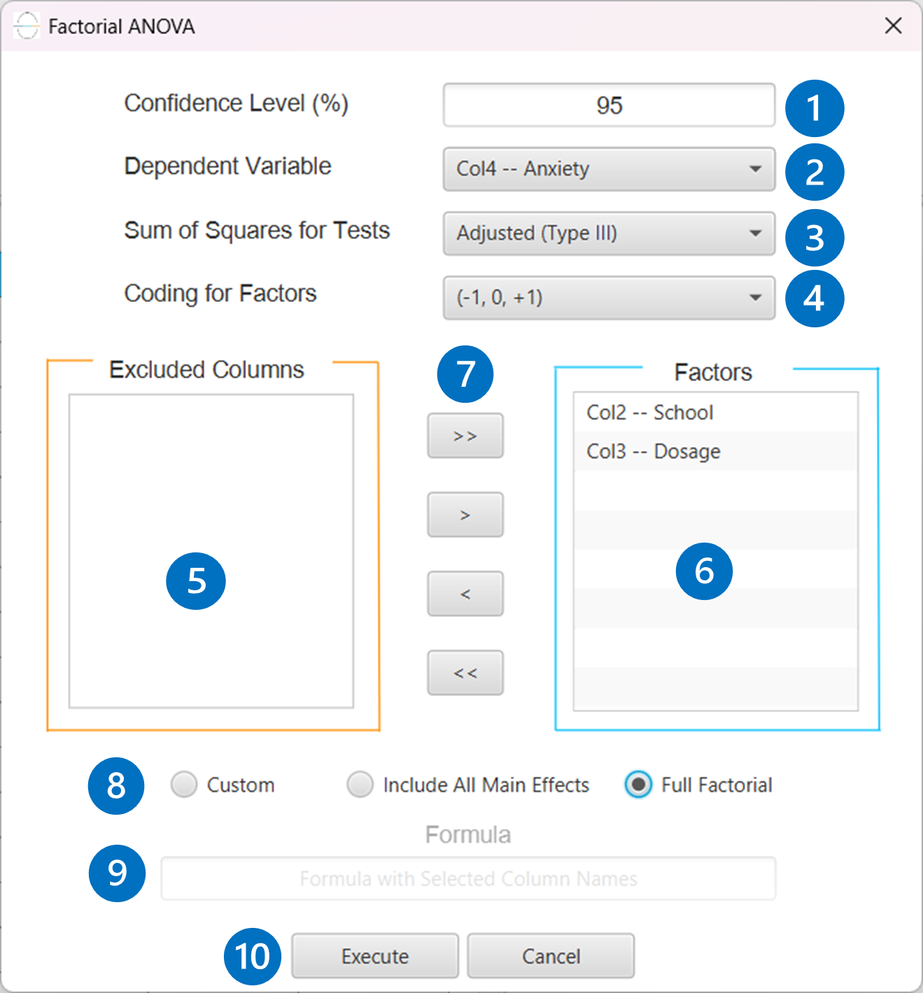
Configuration
- Select
Statistics→Analysis of (Co)Variance→Factorial ANOVA. - Specify the
Confidence Level (%)[1] for the test. - Select the
Dependent Variable[2]. - Select the
Sum of Squaresfor Tests [3]. - Select
Coding for Factors[4]. - Select the columns by clicking on the arrow buttons [7] and moving columns between the
Excluded Columns[5] andFactors[6] lists. - If the (1,0) coding is selected,
Specify Reference Levels[8] for the categorical factors. - Select the prefered
Formula Type[9]. Specify Custom Model Formula[10] for the analysis ifCustomoption is selected. How to specify a custom model formula?- Click on the Execute button [11] to perform the Factorial ANOVA method.
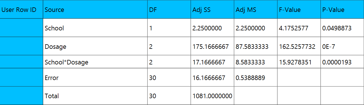
Output
A table analyzing the variance/covariance of each term in the formula is outputted in the output spreadsheet.
ANCOVA
ANCOVA (ANalysis of COVAriance) is a statistical technique that combines features from ANOVA and linear regression. It can be considered extension of ANOVA aimed at including one or more continuous variables that predict the outcome (dependent variable) as well as the categorical factors, usually included in ANOVA. These predictors, known as covariates, are usually not part of the main experimental manipulation but they have an influence on the dependent variable. The inclusion of covariates in an ANOVA model can reduce within-group error variance, as the covariates may be able to explain some of the “unexplained” variance of the model, meaning the variance that cannot be explained by the categorical variables. Moreover, covariates can aid eliminating potential confounds, meaning that whenever a variable is found to influence the dependent variable in a systematic way, it can be included in the model as a covariate in order to remove the bias inflicted by it. A key assumption required in ANCOVA is the homogeneity of regression slopes — this means that the relationship between the covariate(s) and the dependent variable is assumed to be the same across all groups defined by the categorical independent variable. In simpler terms, the effect of the covariate should not vary depending on the level of the factor.
However, this assumption only holds when the model does not include an interaction between the covariate(s) and the factor(s). If you suspect that the effect of the covariate differs by group, you can include an interaction term (e.g., covariate × group) in the model. Doing so allows the regression slopes to vary across groups, and the ANCOVA becomes a test of whether the covariate’s relationship with the outcome is moderated by group membership. Including such an interaction effectively changes the model into a non-parallel slopes model and moves it beyond the traditional ANCOVA framework. It is more flexible but requires sufficient data in each group to reliably estimate group-specific slopes. In ANCOVA, the significance of covariates, factors, and their interactions can be assessed using different methods for calculating sums of squares, most commonly Type I (sequential) and Type III (adjusted) sums of squares.
- Type I Sum of Squares (Sequential): This method adds terms to the model one at a time in a specified order. The sum of squares for each term is calculated as the incremental reduction in the residual sum of squares (SSE) when the term is added to the model. This approach is order-dependent, meaning the significance of each term can vary depending on the order in which variables are entered. Type I SS is often used in balanced designs or when the order of predictors has a meaningful interpretation (e.g., hierarchical regression).
- Type III Sum of Squares (Adjusted): This method evaluates each term after accounting for all other terms in the model, including interactions. It tests each main effect or interaction as if it were the last term added to the model. This is particularly useful in unbalanced designs or when interpreting effects independently of the order in which variables were entered. Type III SS is commonly used in ANCOVA because it allows In both approaches, the significance of a model term (factor, covariate, or interaction) is assessed using an F-test, which compares the two models, the reduced and the full one:
Where:
- \(SSE_{reduced}\) is the sum of squared errors for the reduced (simpler) model.
- \(SSE_{full}\) is the SSE for the full (more complex) model.
- \(df_{reduced}\), \(df_{full}\) are the residual degrees of freedom for the reduced and full models, respectively.
- The numerator measures the reduction in error when moving from the reduced to the full model, adjusted for the number of parameters added.
- The denominator is the mean squared error of the full model.
Use ANCOVA by browsing in the top ribbon:
| Statistics \(\rightarrow\) Analysis of (Co)Variance \(\rightarrow\) ANCOVA |
Input
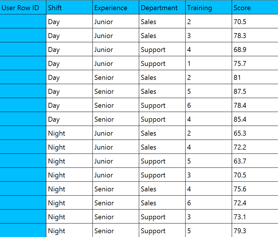
Numerical values should be specified in the input datasheet. The ANCOVA design should include at least one covariate, therefore at least two columns should be specified in the input sheet, one for the dependent variable and one for the covariate.
Configuration
| Confidence Level (%) | Specify the confidence level of the analysis. Values should range from 0 to 100 and correspond to percentages. |
| Dependent Variable | Select the column that corresponds to values of the dependent variable. |
| Sum of Squares for Tests | Select method for calculating the significance of factors, covariates and interactions from the two options provided : Adjusted (Type III), Sequential (Type I). When Sequential (Type I) SS is selected be cautious as the order of terms affects the results of the method. When Include Main Effects or Full Factorial formula options are selected, terms are added in the same order as they appear in the configuration window. If you need a specific order, please use the ‘Custom’ formula option. |
| Coding for Factors | Select the type of coding used to code categorical factors from the two options provided: (-1,0,+1), (1,0) |
| Factors/ Covariates / exclude columns | Select manually the columns that correspond to factors and the columns that correspond to covariates through the dialog window: Use the buttons to move columns between the Factors and Covariates list and Excluded Columns list. Single-arrow buttons will move all selected columns and double-arrow buttons will move all columns. At least one covariate column should be specified. |
| Specify Reference Levels | If the (1,0) coding is selected, specify the reference level for each of the categorical factors specified. The default option for each factor is its last level. |
| Formula Type | These options refer to the terms that will be included in the model. The Custom option allows the user to input a formula defining the exact terms to be included. The Main Effects option allows the analysis of a model that only includes all main effects and finally, the Full Factorial option includes both all main effects and all possible interaction terms to build a full model. |
| Specify Custom Model Formula | Specify the model formula used for the analysis if the Custom option is selected. The formula is created in the Custom Formula Creation dialog window by selecting factors and covariates and adding interaction terms up to the required order. Main effects of the included columns are always part of the model and cannot be excluded. |
Output
The output includes a table summarizing the analysis of variance/covariance. For each term specified in the model formula — including factors, covariates, and interaction terms — the following information is provided:
- Source: The name of the factor, covariate, or interaction term.
- Degrees of Freedom (DF): The number of degrees of freedom associated with the term.
- Sum of Squares (SS): The variation attributed to the term, either adjusted (Type III) or sequential (Type I), depending on the method used.
- Mean Square (MS): The sum of squares divided by the degrees of freedom for the term.
- F-statistic: The ratio of the mean square of the term to the mean square of the residuals, used to test the statistical significance of the term.
- P-value: The probability of observing an F-statistic as extreme as the one calculated, assuming the null hypothesis is true.
- Significant: A binary column specifying whether the term is significant based on the specified confidence level and the calculated P-value.
Example
Input
In the input datasheet the requirement is to specify at least two columns and insert the appropriate data, as shown below.
Configuration
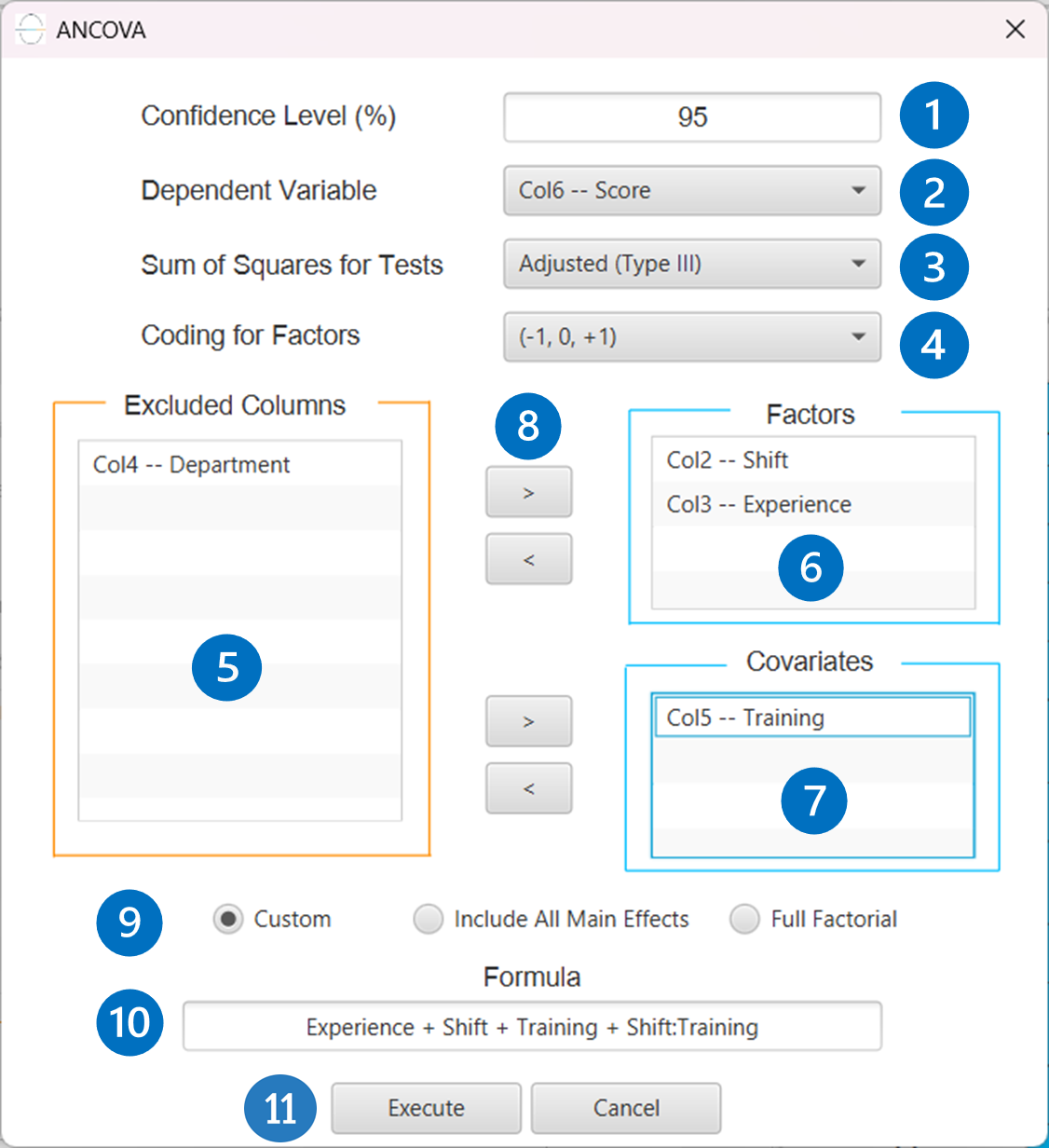
- Select
Statistics→Analysis of (Co)Variance→ANCOVA. - Specify the
Confidence Level (%)[1] for the test. - Select the
Dependent Variable[2]. - Select the
Sum of Squaresfor Tests [3]. - Select
Coding for Factors[4]. - Select the columns by clicking on the arrow buttons [8] and moving columns between the
Excluded Columns[5] andFactors[6] andCovariates[7] lists. - If the (1,0) coding is selected,
Specify Reference Levels[9] for the categorical factors. - Select the prefered
Formula Type[10]. Specify Custom Model Formula[11] for the analysis ifCustomoption is selected. How to specify a custom model formula?- Click on the
Executebutton [12] to perform the ANCOVA method.
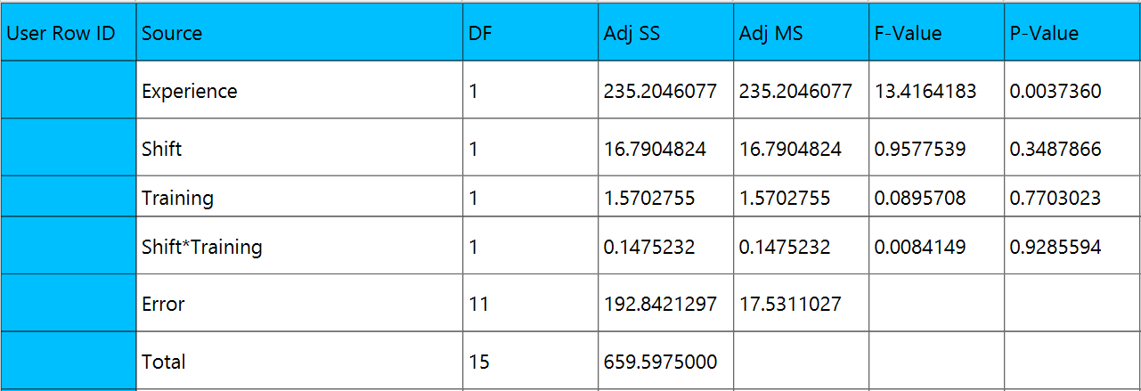
Output
A table analyzing the variance/covariance of each term in the formula is outputted in the output spreadsheet.
MANOVA
Multivariate Analysis of Variance (MANOVA) is a statistical method used to determine whether one or more independent variables (groups) have a significant effect on two or more dependent variables simultaneously. Unlike ANOVA, which analyzes only one dependent variable at a time, MANOVA considers the relationships among multiple dependent variables and tests for overall differences in outcome profiles across groups. The process begins by estimating the mean vectors of the dependent variables for each group defined by the independent variable. The model then partitions the total variation in the data into two sources: between-group variation, which reflects differences across groups, and within-group variation, which represents random variability within each group. MANOVA essentially evaluates whether the combination of dependent variables exhibits different mean patterns between groups. If a significant overall difference is detected, the analysis can proceed with separate univariate ANOVA tests on each dependent variable to identify which ones contribute most to the observed effect. The validity of MANOVA relies on certain assumptions, including multivariate normality, homogeneity of variance-covariance matrices, and independent observations.
Use MANOVA by browsing in the top ribbon:
| Statistics \(\rightarrow\) Analysis of (Co)Variance \(\rightarrow\) MANOVA |
Input
Numerical values should be specified in the input datasheet. The MANOVA design requires at least one factor and two or more dependent variables. Please ensure the input sheet contains one categorical column for the factor and at least two numeric columns for the dependent variables.
Configuration
| Confidence Level (%) | Specify the confidence level of the analysis. Values should range from 0 to 100 and correspond to percentages. |
| Sum of Squares for Tests | Select method for calculating the significance of factors, covariates and interactions from the two options provided : Adjusted (Type III), Sequential (Type I). When Sequential (Type I) SS is selected be cautious as the order of terms affects the results of the method. When Include Main Effects or Full Factorial formula options are selected, terms are added in the same order as they appear in the configuration window. If you need a specific order, please use the ‘Custom’ formula option. |
| Coding for Factors | Select the type of coding used to code categorical factors from the two options provided: (-1,0,+1), (1,0) |
| Factors/ Dependent Variables / exclude columns | Select manually the columns that correspond to factors and the columns that correspond to dependent variables through the dialog window. Use the arrow buttons to move columns between the Excluded Columns list and the Factors or Dependent Variables fields. The single-arrow buttons move selected columns. For a valid MANOVA design, you must specify at least one factor and two or more dependent variables. |
| Specify Reference Levels | If the (1,0) coding is selected, specify the reference level for each of the categorical factors specified. The default option for each factor is its last level. |
| Formula Type | These options refer to the terms that will be included in the model. The Custom option allows the user to input a formula defining the exact terms to be included. The Main Effects option allows the analysis of a model that only includes all main effects and finally, the Full Factorial option includes both all main effects and all possible interaction terms to build a full model. |
| Specify Custom Model Formula | Specify the model formula used for the analysis if the Custom option is selected. The formula is created in the Custom Formula Creation dialog window by selecting factors and covariates and adding interaction terms up to the required order. Main effects of the included columns are always part of the model and cannot be excluded. |
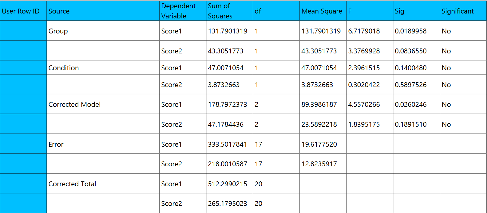
Output
The output includes a table summarizing the analysis of variance/covariance. For each term specified in the model formula — including factors and interaction terms — the following information is provided:
- Source: The name of the factor, covariate, or interaction term.
- Dependent Variable: Indicates the name of the outcome variable being analyzed in the current test.
- Degrees of Freedom (DF): The number of degrees of freedom associated with the term.
- Sum of Squares (SS): The variation attributed to the term, either adjusted (Type III) or sequential (Type I), depending on the method used.
- Mean Square (MS): The sum of squares divided by the degrees of freedom for the term.
- F-statistic: The ratio of the mean square of the term to the mean square of the residuals, used to test the statistical significance of the term.
- P-value: The probability of observing an F-statistic as extreme as the one calculated, assuming the null hypothesis is true.
- Significant: A binary column specifying whether the term is significant based on the specified confidence level and the calculated P-value.
Example
Input
In the input datasheet the requirement is to specify three columns and insert the appropriate data, as shown below.
Configuration
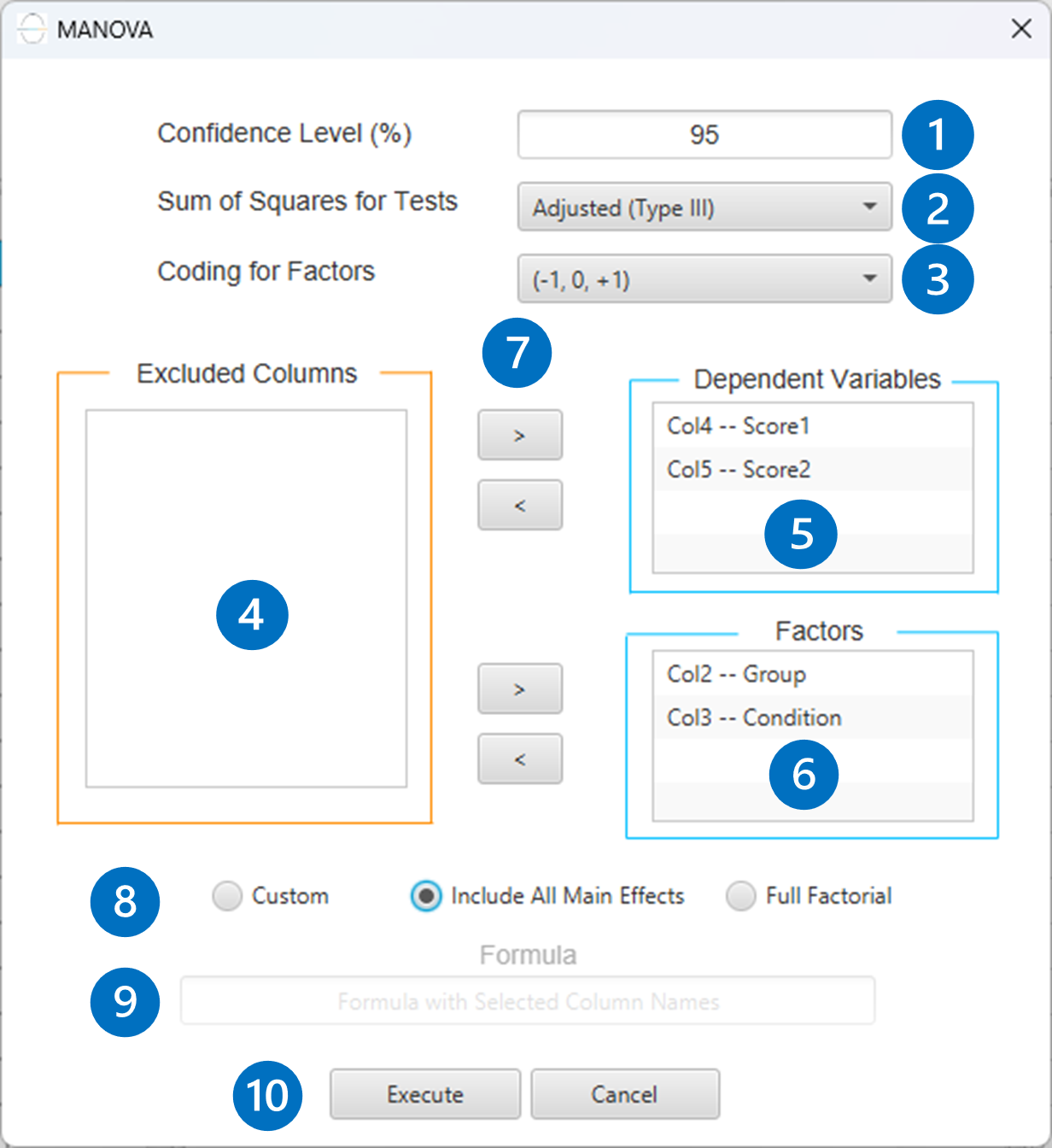
- Select
Statistics\(\rightarrow\)Analysis of (Co)Variance\(\rightarrow\)MANOVA. - Specify the
Confidence Level (%)[1] for the test. - Select the
Sum of Squares for Tests[2]. - Select
Coding for Factors[3]. - Select the columns by clicking on the arrow buttons [7] and moving columns between the
Excluded Columns[4] andDependent Variables[5] andFactors[6] lists. - If the (1,0) coding is selected,
Specify Reference Levels[8] for the categorical factors. - Select the prefered
Formula Type[9]. Specify Custom Model Formula[10] for the analysis ifCustomoption is selected. How to specify a custom model formula?- Click on the
Executebutton [11] to perform the MANOVA method.
Output
A table analyzing the variance/covariance of each term in the formula is outputted in the output spreadsheet.
MANCOVA
MANCOVA (Multivariate Analysis of Covariance) is an extension of MANOVA that allows researchers to examine whether two or more dependent variables differ across levels of one or more independent variables (factors), while statistically controlling for the effects of one or more covariates. Covariates are continuous variables that are not of primary interest but may influence the dependent variables. By adjusting for these covariates, MANCOVA improves the accuracy of the group comparisons and reduces potential error variance. The method first removes the influence of the covariates from the dependent variables through a process called covariate adjustment (essentially a regression step). Then, it performs a multivariate analysis of the residuals to determine whether group differences remain after accounting for the covariates. Like MANOVA, MANCOVA considers the interrelationships among the dependent variables and tests for overall group effects on their combination. MANCOVA assumes multivariate normality, linear relationships between covariates and dependent variables, homogeneity of regression slopes, and equality of covariance matrices across groups. When these assumptions are met, MANCOVA provides a powerful way to control confounding variables and reveal the true effects of the experimental factors.
Use MANCOVA by browsing in the top ribbon:
| Statistics \(\rightarrow\) Analysis of (Co)Variance \(\rightarrow\) MANCOVA |
Input
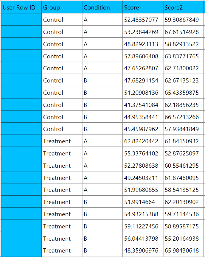
Numerical values should be specified in the input datasheet. To perform a valid MANCOVA, the input must include at least one factor, one or more covariates, and two or more dependent variables. Please ensure the input sheet contains one categorical column for the factor, one or more numeric columns for the covariates, and at least two numeric columns for the dependent variables.
Configuration
| Confidence Level (%) | Specify the confidence level of the analysis. Values should range from 0 to 100 and correspond to percentages. |
| Sum of Squares for Tests | Select method for calculating the significance of factors, covariates and interactions from the two options provided : Adjusted (Type III), Sequential (Type I). When Sequential (Type I) SS is selected be cautious as the order of terms affects the results of the method. When Include Main Effects or Full Factorial formula options are selected, terms are added in the same order as they appear in the configuration window. If you need a specific order, please use the ‘Custom’ formula option. |
| Coding for Factors | Select the type of coding used to code categorical factors from the two options provided: (-1,0,+1), (1,0) |
| Dependent Variables / Covariate/ Factor/ Exclude columns | Select manually the columns that correspond to factors, columns that correspond to covariates and the columns that correspond to dependent variables through the dialog window. Use the arrow buttons to move columns between the Excluded Columns list and the Factors, Covariates or Dependent Variables fields. The single-arrow buttons move selected columns. For a valid MANCOVA design, you must specify at least one factor , one or more covariates and two or more dependent variables. |
| Specify Reference Levels | If the (1,0) coding is selected, specify the reference level for each of the categorical factors specified. The default option for each factor is its last level. |
| Formula Type | These options refer to the terms that will be included in the model. The Custom option allows the user to input a formula defining the exact terms to be included. The Main Effects option allows the analysis of a model that only includes all main effects and finally, the Full Factorial option includes both all main effects and all possible interaction terms to build a full model. |
| Specify Custom Model Formula | Specify the model formula used for the analysis if the Custom option is selected. The formula is created in the Custom Formula Creation dialog window by selecting factors and covariates and adding interaction terms up to the required order. Main effects of the included columns are always part of the model and cannot be excluded. |
Output
The output includes a table summarizing the analysis of variance/covariance. For each term specified in the model formula — including factors, covariates and interaction terms — the following information is provided:
- Source: The name of the factor, covariate, or interaction term.
- Dependent Variable: Indicates the name of the outcome variable being analyzed in the current test.
- Degrees of Freedom (DF): The number of degrees of freedom associated with the term.
- Sum of Squares (SS): The variation attributed to the term, either adjusted (Type III) or sequential (Type I), depending on the method used.
- Mean Square (MS): The sum of squares divided by the degrees of freedom for the term.
- F-statistic: The ratio of the mean square of the term to the mean square of the residuals, used to test the statistical significance of the term.
- P-value: The probability of observing an F-statistic as extreme as the one calculated, assuming the null hypothesis is true.
- Significant: A binary column specifying whether the term is significant based on the specified confidence level and the calculated P-value.
Example
Input
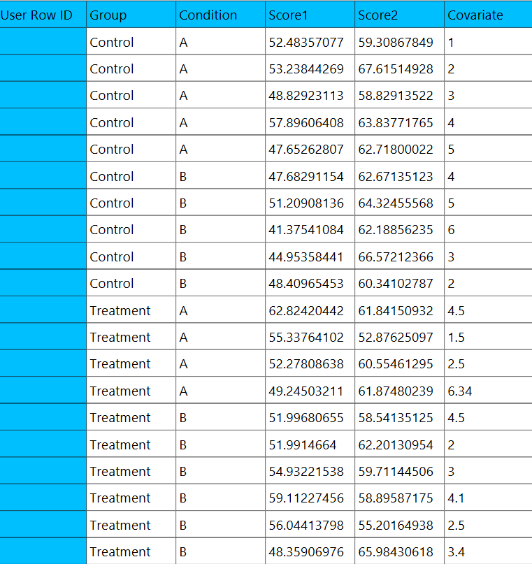
In the input datasheet the requirement is to specify three columns and insert the appropriate data, as shown below.
Configuration
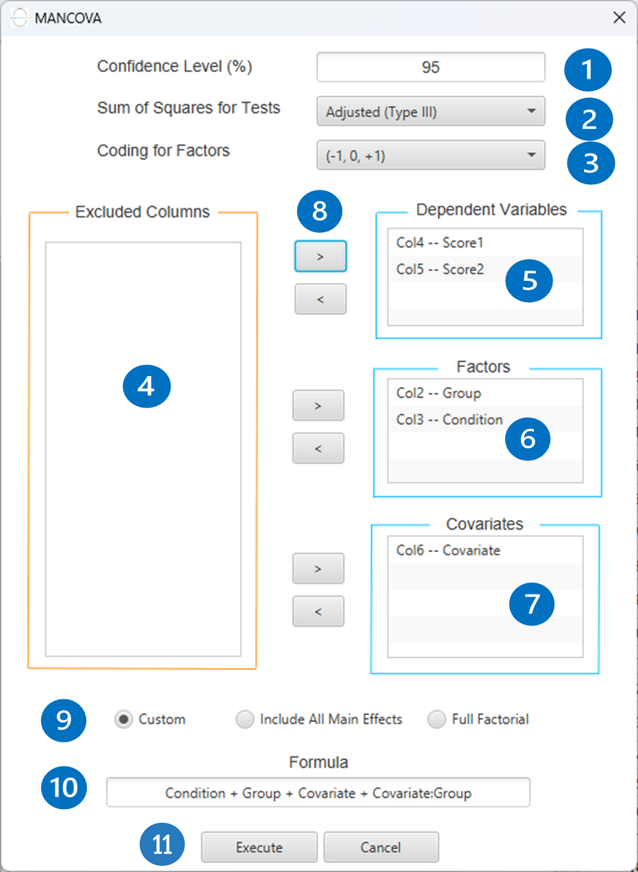
- Select
Statistics\(\rightarrow\)Analysis of (Co)Variance\(\rightarrow\)MANCOVA. - Specify the
Confidence Level (%)[1] for the test. - Select the
Sum of Squares for Tests[2]. - Select
Coding for Factors[3]. - Select the columns by clicking on the arrow buttons [8] and moving columns between the
Excluded Columns[4],Dependent Variables[5],Factors[6] andCovariates[7] lists. - If the (1,0) coding is selected,
Specify Reference Levels[9] for the categorical factors. - Select the prefered
Formula Type[10]. Specify Custom Model Formula[11] for the analysis ifCustomoption is selected. How to specify a custom model formula?- Click on the
Executebutton [12] to perform the MANCOVA method.
Output
A table analyzing the variance/covariance of each term in the formula is outputted in the output spreadsheet.
Repeated Measures
The Repeated Measures ANOVA, or within-subject ANOVA is a statistical method used to analyze groups of related dependent variables, that represent different measurements of the same attribute. Unlike traditional ANOVA, which assumes independent observations across groups, repeated measures ANOVA accounts for the correlated nature of the data that arises when the same subjects contribute multiple observations. This method is widely used in experiments where each subject is tested repeatedly across different conditions or in different time points. These conditions, time points or tasks are the repeated measures of the analysis and are called the within-subjects factor(s) while between-subject factors are the traditional grouping variables or factors used in ANOVA experiments. A repeated measures ANOVA partitions the total variance into:
- Between-subjects variance: Differences between participants’ overall levels
- Within-subjects variance: Differences due to the repeated measures factor(s)
- Error Variance: Unexplained variability not attributed to condition or subject effects.
Use Repeated Measures ANOVA by browsing in the top ribbon:
| Statistics \(\rightarrow\) Analysis of (Co)Variance \(\rightarrow\) RM ANOVA |
Input
Numerical values should be specified in the input datasheet. The Repeated Measures ANOVA design requires three columns to specified as input. One designated for within-subjects, one for the subjects and one for the dependent variable.
Configuration
| Confidence Level (%) | Specify the confidence level of the analysis. Values should range from 0 to 100 and correspond to percentages. |
| Sum of Squares for Tests | Select method for calculating the significance of factors, covariates and interactions from the two options provided : Adjusted (Type III), Sequential (Type I). |
| Subject Column | Select the column that specifies the subjects. |
| Within Column | Select the column that corresponds to the repeated measures. |
| Dependent Variable | Select the column that corresponds to values of the dependent variable. |
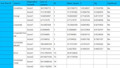
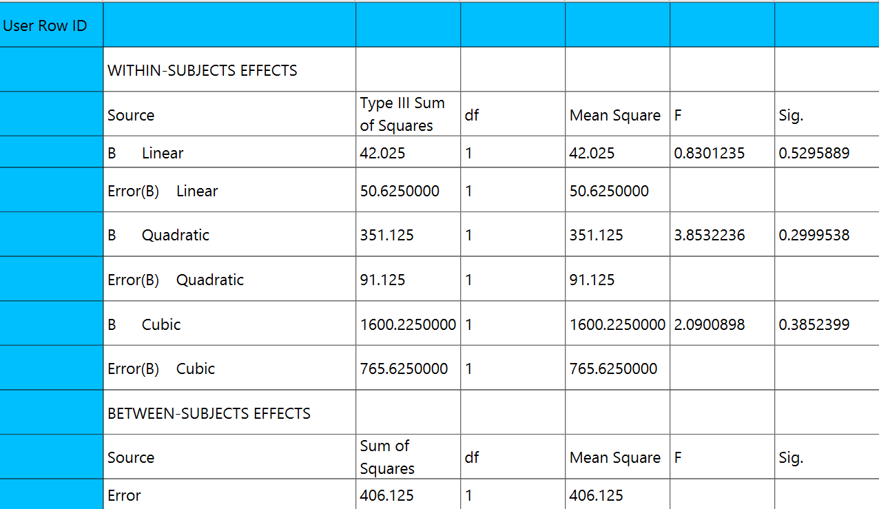
Output
The output includes two tables summarizing the analysis of variance for within-subjects and between-subjects effects. For each effect tested — including within-subjects factors, polynomial contrasts (e.g., linear, quadratic), interactions, and between-subjects variables — the following information is provided:
- Source: The name of the factor, covariate, or interaction term.
- Degrees of Freedom (DF): The number of degrees of freedom associated with the term.
- Sum of Squares (SS): The variation attributed to the term, either adjusted (Type III) or sequential (Type I), depending on the method used.
- Mean Square (MS): The sum of squares divided by the degrees of freedom for the term.
- F-statistic: The ratio of the mean square of the term to the mean square of the residuals, used to test the statistical significance of the term.
- P-value: The probability of observing an F-statistic as extreme as the one calculated, assuming the null hypothesis is true.
- Significant: A binary column specifying whether the term is significant based on the specified confidence level and the calculated P-value.
Example
Input
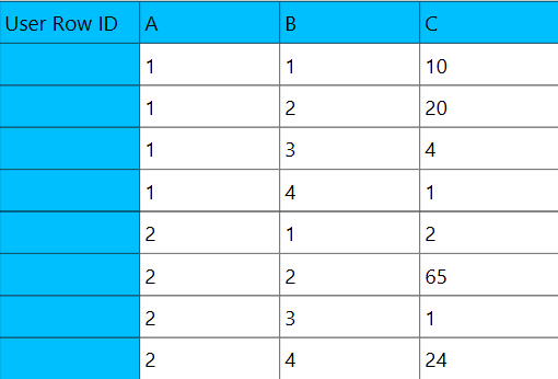
In the input datasheet the requirement is to specify three columns and insert the appropriate data, as shown below.
Configuration
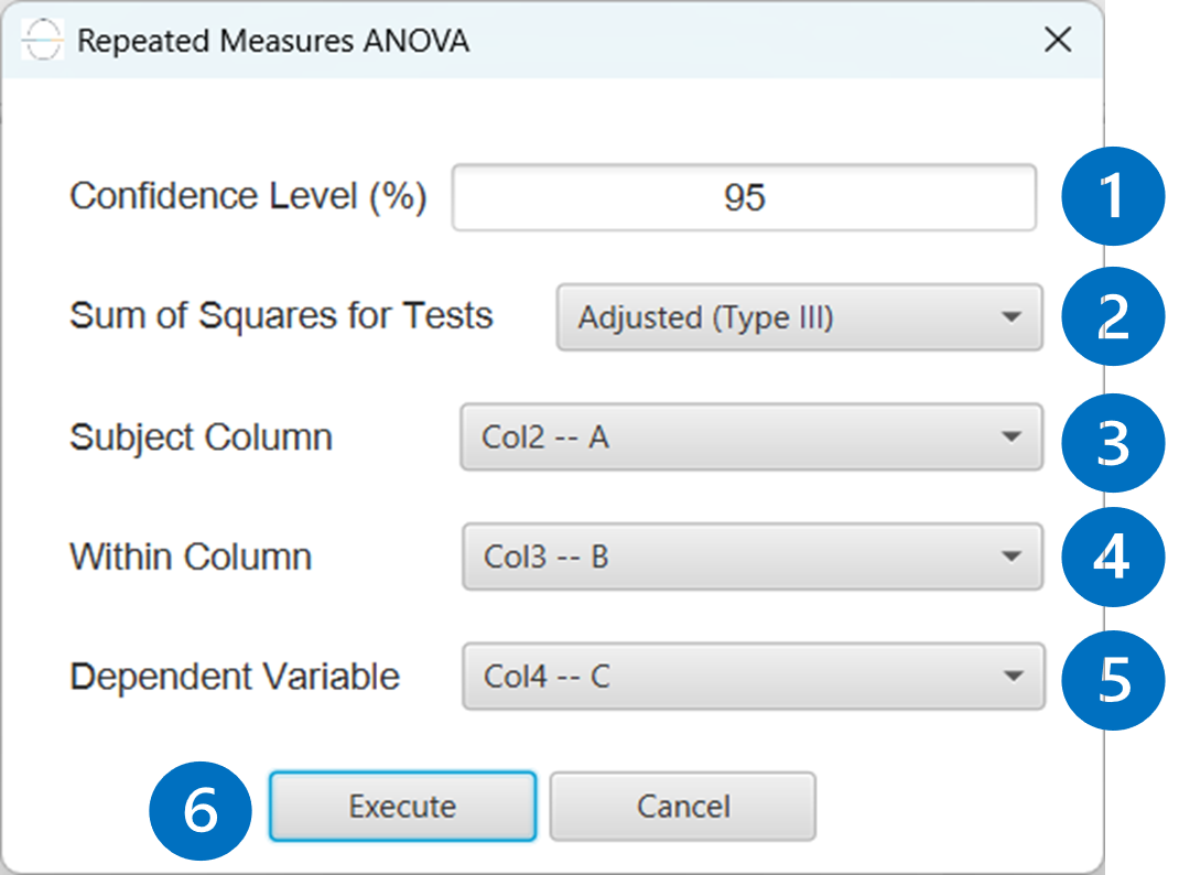
- Select
Statistics→Analysis of (Co)Variance→RM ANOVA. - Specify the
Confidence Level (%)[1] for the test. - Select the
Sum of Squaresfor Tests [2]. - Select the
Subject Column[3]. - Select the
Within Column[4]. - Select the
Dependent Variable[5]. - Click on the
Executebutton [6] to perform the Repeated Measures ANOVA method.
Output
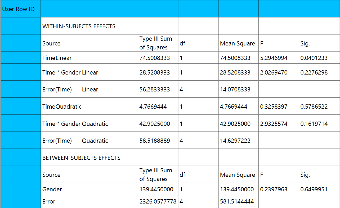
The two tables analyzing the within-subject effects and the between-subject effects are shown in the output spreadsheet.
Mixed ANOVA
Mixed ANOVA is a statistical method used to analyze data that involve both within-subjects and between-subjects factors or covariates. It is particularly useful in experimental designs where each subject is measured repeatedly across different conditions and where different groups of subjects are exposed to different treatments or categories. Unlike Repeated Measures ANOVA, which only considers measurements taken repeatedly from the same subjects, a mixed ANOVA accommodates both the correlated nature of repeated measurements and the independence of observations across groups. In a mixed ANOVA, the within-subjects factor(s) represent repeated measurements (such as time points, conditions, or tasks), while the between-subjects factor(s) capture traditional group differences (such as gender, treatment group, or experimental condition). In addition, mixed ANOVA designs can include between-subject covariates, which are continuous variables (e.g., age, baseline performance, socioeconomic status) that may influence the dependent variable but are not of primary experimental interest. Incorporating these covariates helps control for individual differences, reduce error variance, and provide a clearer estimate of the effects of both within- and between-subject factors.
A mixed ANOVA partitions the total variance into:
- Between-subjects variance: Differences due to group membership (e.g., treatment vs. control)
- Within-subjects variance: Differences within individuals across repeated conditions or time points
- Interaction variance: Variability due to the interaction between within-subjects and between-subjects factors
- Error variance: Unexplained variability not attributed to condition, group, or their interaction
Use Mixed ANOVA by browsing in the top ribbon:
| Statistics \(\rightarrow\) Analysis of (Co)Variance \(\rightarrow\) Mixed ANOVA |
Input
Numerical values should be specified in the input datasheet. The Mixed ANOVA design requires four column to specified as input. One designated for within-subjects, one for the subjects, one for between-subjects and one for the dependent variable.
Configuration
| Confidence Level (%) | Specify the confidence level of the analysis. Values should range from 0 to 100 and correspond to percentages. |
| Sum of Squares for Tests | Select method for calculating the significance of factors, covariates and interactions from the two options provided : Adjusted (Type III), Sequential (Type I). When Sequential (Type I) SS is selected be cautious as the order of terms affects the results of the method. When Include Main Effects or Full Factorial formula options are selected, terms are added in the same order as they appear in the configuration window. If you need a specific order, please use the ‘Custom’ formula option. |
| Coding for Factors | Select the type of coding used to code categorical factors from the two options provided: (-1,0,+1), (1,0) |
| Subject Column | Select the column that specifies the subjects. |
| Within Column | Select the column that corresponds to the repeated measures. |
| Dependent Variable | Select the column that corresponds to values of the dependent variable. |
| Between-Subjects Factors/ Covariates / exclude columns | Select manually the columns that correspond to between-subject factors and the columns that correspond to covariates through the dialog window: Use the buttons to move columns between the Between-Subjects Factors and Covariates list and Excluded Columns list. Single-arrow buttons will move all selected columns and double-arrow buttons will move all columns. At least one between-subject or one covariate column should be specified. |
| Specify Reference Levels | If the (1,0) coding is selected, specify the reference level for each of the categorical between-subjects factors specified. The default option for each factor is its last level. |
| Formula Type | These options refer to the terms that will be included in the model. The Custom option allows the user to input a formula defining the exact terms to be included. The Main Effects option allows the analysis of a model that only includes all main effects and finally, the Full Factorial option includes both all main effects and all possible interaction terms to build a full model. |
| Specify Custom Model Formula | Specify the model formula used for the analysis if the Custom option is selected. The formula is created in the Custom Formula Creation dialog window by selecting factors and covariates and adding interaction terms up to the required order. Main effects of the included columns are always part of the model and cannot be excluded. |
Output
The output includes two tables summarizing the analysis of variance for within-subjects and between-subjects effects. For each effect tested — including within-subjects factors, polynomial contrasts (e.g., linear, quadratic), interactions, and between-subjects variables — the following information is provided:
- Source: The name of the factor, interaction, or trend component (e.g., linear, quadratic) being tested.
- Degrees of Freedom (DF): The number of degrees of freedom associated with the term.
- Sum of Squares (SS): The variation attributed to the term, either adjusted (Type III) or sequential (Type I), depending on the method used.
- Mean Square (MS): The sum of squares divided by the degrees of freedom for the term.
- F-statistic: The ratio of the mean square of the term to the mean square of the residuals, used to test the statistical significance of the term.
- P-value: The probability of observing an F-statistic as extreme as the one calculated, assuming the null hypothesis is true.
- Significant: A binary column specifying whether the term is significant based on the specified confidence level and the calculated P-value.
Example
Input
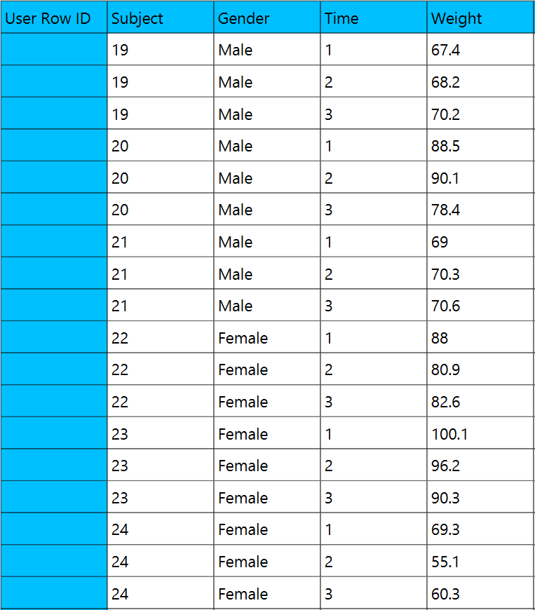
In the input datasheet the requirement is to specify four columns and insert the appropriate data, as shown below.
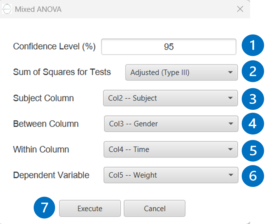
Configuration
- Select
Statistics→Analysis of (Co)Variance→Mixed ANOVA. - Specify the
Confidence Level(%) [1] for the test. - Select the
Sum of Squaresfor Tests [2]. - Select the
Subject Column[3]. - Select the
Within Column[4]. - Select the
Dependent Variable[5]. - Select the columns by clicking on the arrow buttons [10] and moving columns between the
Excluded Columns[7] andBetween-Subjects Factors[8] andCovariates[9] lists. - If the (1,0) coding is selected,
Specify Reference Levels[11] for the categorical factors. - Select the prefered
Formula Type[12]. Specify Custom Model Formula[13] for the analysis ifCustomoption is selected. How to specify a custom model formula?- Click on the
Executebutton [14] to perform Mixed ANOVA.
Output
The two tables analyzing the within-subject effects and the between-subject effects are shown in the output spreadsheet.
Specify Custom Model Formula
The Custom formula option allows the user to define the exact model terms to be included in the analysis. This is useful when a specific combination of main effects and interaction terms is required, instead of using the predefined Main Effects or Full Factorial options.
The custom formula is specified through the Custom Formula Creation dialog window. This window is used to construct the model by selecting factors and covariates and adding terms and interactions up to the desired order. The resulting formula is shown automatically in the formula display area at the bottom of the dialog.
Only factors and covariates are used in this dialog window. Main effects are always included for the columns present in the Included Columns list and cannot be excluded. Therefore, a valid custom formula always contains at least one main effect.
Dialog window components
| Included Columns | Displays the factors and covariates available for the custom formula. If a column appears in this list, its main effect is included by default in the model. |
| Included Terms | Displays the terms currently included in the model formula, including main effects and interaction terms. |
| Add interactions (up to order) | Adds all possible interaction terms among the selected columns up to the specified order. |
| Add terms (up to order) | Adds all terms up to the specified order for the selected columns. This includes the main effects and all interaction terms up to that order. |
| Add Custom Interaction | Adds only the specific interaction defined by the selected columns. |
| Delete Selected | Removes the selected interaction term or terms from the Included Terms list. Main effects cannot be removed. |
| Reset Selections | Restores the formula to its initial state. |
| Move up / Move down | Changes the order of the terms in the Included Terms list. This is important when Sequential (Type I) sum of squares is selected, since the order of terms affects the results. |
| Formula display area | Displays the custom model formula exactly as it will be used in the analysis. |
References
- Rutherford, A. (2011). ANOVA and ANCOVA: a GLM approach. John Wiley & Sons.
- Huberty, C. J., & Olejnik, S. (2007). Applied MANOVA and discriminant analysis. John Wiley & Sons.
- Cohen, B. H. (2002). Calculating a factorial ANOVA from means and standard deviations. Understanding Statistics: Statistical Issues in Psychology, Education, and the Social Sciences, 1(3), 191-203.
Version History
Introduced in Isalos Analytics Platform v1.0.0
Instructions last updated on May 2025