Curve Fitting

Curve fitting is the process of estimating model parameters so a mathematical function best represents an observed relationship between an independent variable \(X\) and a dependent response \(𝑌\). In practice, you choose a model form (e.g., linear, polynomial, exponential, or mechanistic models such as Hill-type dose–response curves) and define a criterion for “best”. The most common criterion is least squares, where parameters are selected to minimize the sum of squared residuals \(r_i = y_i - \hat{y_i}\). Depending on the model, fitting can be done with linear regression (closed-form solutions) or nonlinear regression (iterative optimization). When the response variance is not constant across \(X\), weighted least squares is often used so points with lower variance (higher confidence) influence the fit more than noisier points.

Different curve fitting methods make different assumptions and trade-offs. Nonlinear least squares is widely used for dose–response because it directly estimates interpretable parameters, but it can be sensitive to starting values, local minima, and parameter correlation—especially in multi-parameter models. Robust regression reduces the influence of outliers, while regularization or constraints (fixing slopes, bounding parameters) can stabilize fits when data are sparse or noisy. Good practice is to evaluate fit quality using residual plots, confidence intervals, and goodness-of-fit metrics (e.g., \(R^2\)), and to prefer models that are both statistically adequate and biologically/chemically plausible rather than simply the most flexible.

This section is organized into two subsections that reflect the main families of curve fitting used in this framework. The first subsection covers nonlinear equations, where model parameters are estimated using the Levenberg–Marquardt algorithm. The second subsection focuses on Lethal Concentration/Dose (LCx/LDx) analysis, which relies on probit regression solved using the Newton–Raphson method. The theoretical basis, assumptions, and practical implications of each approach are described in detail in their respective sections.

---

Non Linear Equations

In this context, a nonlinear equation is any model where the predicted response \(\hat{Y}\) depends on parameters in a way that cannot be rewritten as a linear combination of those parameters. Formally, you model the relationship as

\begin{equation} Y_i = f(X_i,\theta) + \epsilon_i \end{equation}

where \(f(⋅)\) is a chosen functional form (e.g., Hill-type dose–response, exponential growth/decay, biphasic/bell-shaped models), \(\theta\) is the vector of unknown parameters, and \(\epsilon_i\) represents measurement noise and unexplained variability. “Nonlinear” here refers to the parameters, not necessarily the curve shape: a model can be curved but still linear-in-parameters (e.g., polynomial regression), whereas dose–response models are typically nonlinear because parameters appear inside exponents, ratios, or both. Because there is no closed-form solution for \(\theta\), parameters are estimated by numerical optimization, most commonly by minimizing an objective function such as the sum of squared residuals:

\begin{equation} S(\theta) = \sum_{i=1}^n w_i(Y_i - f(X_i,\theta))^2 \end{equation}

with \(w_i = 1\) for ordinary least squares.

To estimate parameters for these nonlinear least-squares models, Isalos uses the Levenberg–Marquardt (LM) algorithm. LM is an iterative method designed specifically for minimizing sums of squared residuals. It updates the parameter vector \(\theta\) by using the model’s Jacobian (sensitivities of predictions to parameters) to propose a step that improves the fit. Intuitively, LM blends two behaviors: when the current estimate is close to the optimum and the model is locally well-approximated by a quadratic surface, LM behaves like Gauss–Newton (fast convergence); when the problem is ill-conditioned or far from the optimum, LM increases a damping term and behaves more like gradient descent (more stable steps). This balance makes LM a good default for dose–response-type equations: these models are naturally expressed as least-squares problems, usually have a moderate number of parameters, and benefit from an algorithm that is both efficient near the solution and robust when initial guesses are imperfect or parameters are correlated.

After fitting, parameter uncertainty is commonly summarized with confidence intervals. Symmetrical (Wald-type) confidence intervals use the local curvature of the objective function at the optimum—via the approximate covariance matrix derived from the Jacobian—to produce intervals of the form \(\hat{\theta}_j \pm tSE(\hat{\theta}_j)\). They are fast and work well when the estimator is approximately normal and the loss surface is locally symmetric. Profile likelihood confidence intervals are more computationally intensive but often more reliable for nonlinear models: each parameter \(\theta_j\) is fixed across a grid of values, the remaining parameters are re-optimized, and the interval is defined by the set of values that worsen the fit by no more than a threshold . In practice, if symmetric and profile intervals are similar, the parameter is usually well-identified; if they differ substantially (profile intervals asymmetric or much wider), that signals strong nonlinearity, parameter correlation, boundary effects, or limited information in the data—conditions where symmetric intervals can be misleadingly optimistic.

The remainder of this nonlinear-equation section is organized into three practical cases, based on how many dependent variables (response columns) the model is fitted to. First, we cover models fitted to a single dependent variable (Y column). Next, we extend the workflow to models that simultaneously fit two dependent variables (two Y columns), typically sharing one or more parameters. Finally, we address multiple dependent variables, where the same model framework is applied across several responses in parallel (often with global/shared parameters). Each case is accompanied by dedicated, instructions and examples to show the setup.

Fit your data using the Non Linear Equations function by browsing in the top ribbon:

Statistics \(\rightarrow\) Curve Fitting \(\rightarrow\) Non Linear Equations

Case 1: One dependent variable

Input

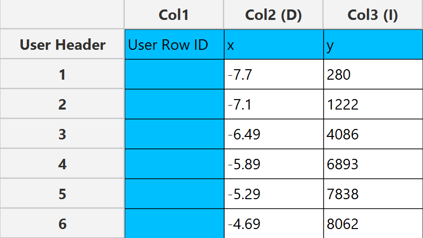
Numerical values should be specified in the input datasheet. The design Non Linear Equations with one dependent variable (Case 1) requires at least two columns in the input sheet: one column representing the independent variable, and another column for the numerical response variable (dependent variable). Columns with empty cells cannot be inculded in the analysis. Each row represents a single observation.

Configuration

Category	Select the model family that best matches your analysis.
Model	Select the specific equation to fit within the chosen category.
Independent Variable	Select the column that corresponds to values of the independent variable.
Dependent Variable	Select the column that corresponds to values of the dependent variable.
Extra Parameters	Enter values for any additional model-specific parameters required for the selected equation. Refer to the documentation for the chosen model (in the list of available models) for the definition, allowed range/options, and recommended settings for each extra parameter.
Confidence Level (%)	Specify the confidence level of the analysis. Values should range from 0 to 100 and correspond to percentages.
Confidence Interval Type	Choose how confidence intervals are computed: Symmetrical, Approximate and Assymetrical(Likelihood).
Logarithmize Independent Variable Data	Use this option to logarithmize (base 10) the data in the specified independent variable column.

Output

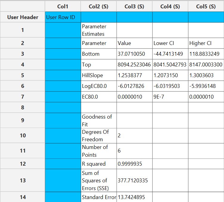
The output spreadsheet contains two tables:

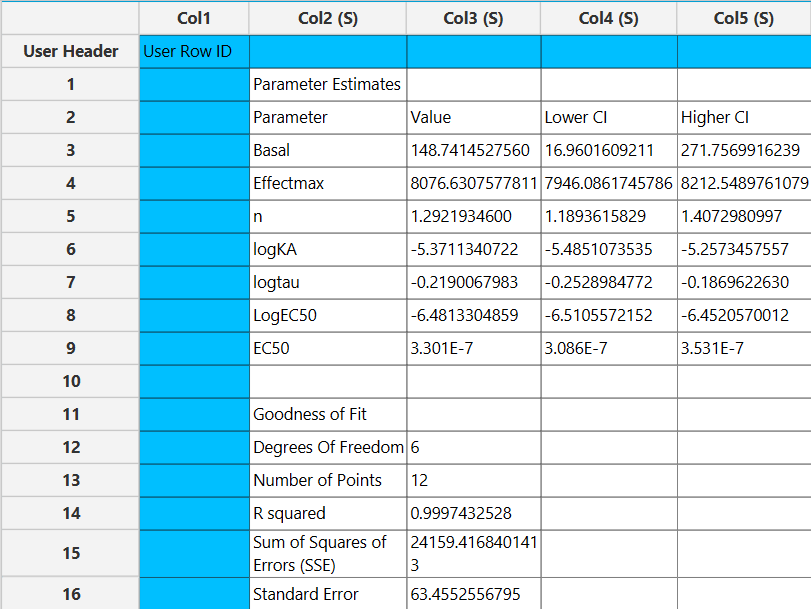
1. Parameter Estimates: Reports the fitted value for each estimated parameter along with the lower and upper confidence limits at the selected confidence level. For parameters expressed on a log scale (e.g., LogEC50), the output also includes the corresponding back-transformed values (e.g., EC50) and their confidence limits.
2. Goodness of Fit: Summarizes overall fit statistics, including the number of data points used, degrees of freedom, residual sum of squares (SS), and the standard error of the regression.

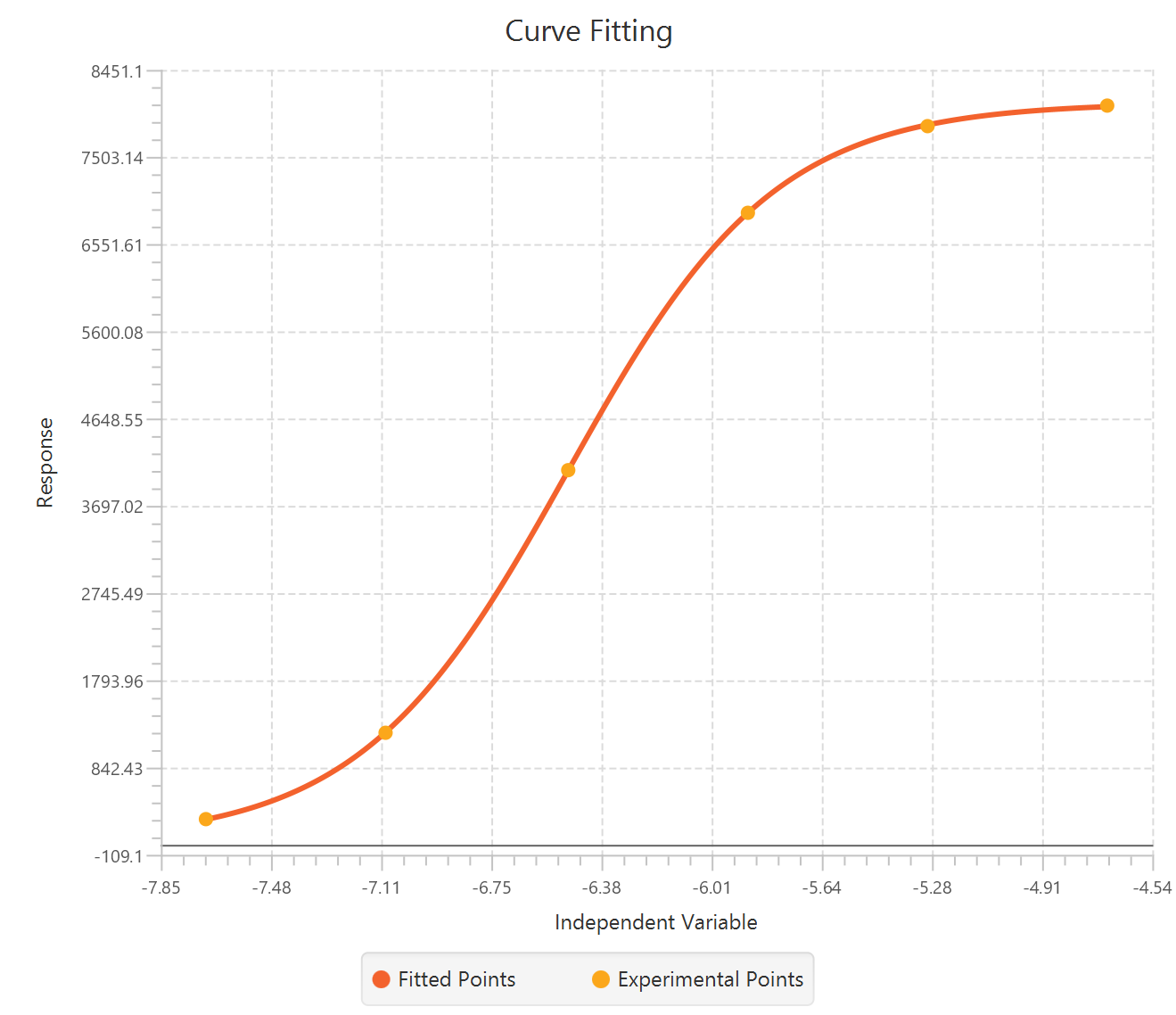
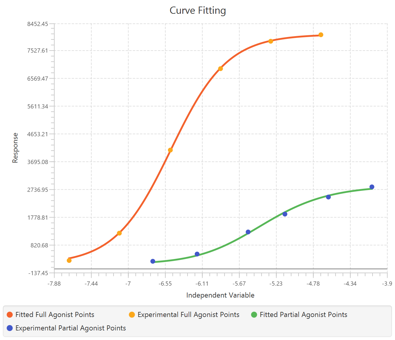
In addition, a pop-up window displays a plot of the fitted curve overlaid with the experimental data points.

Example

Input

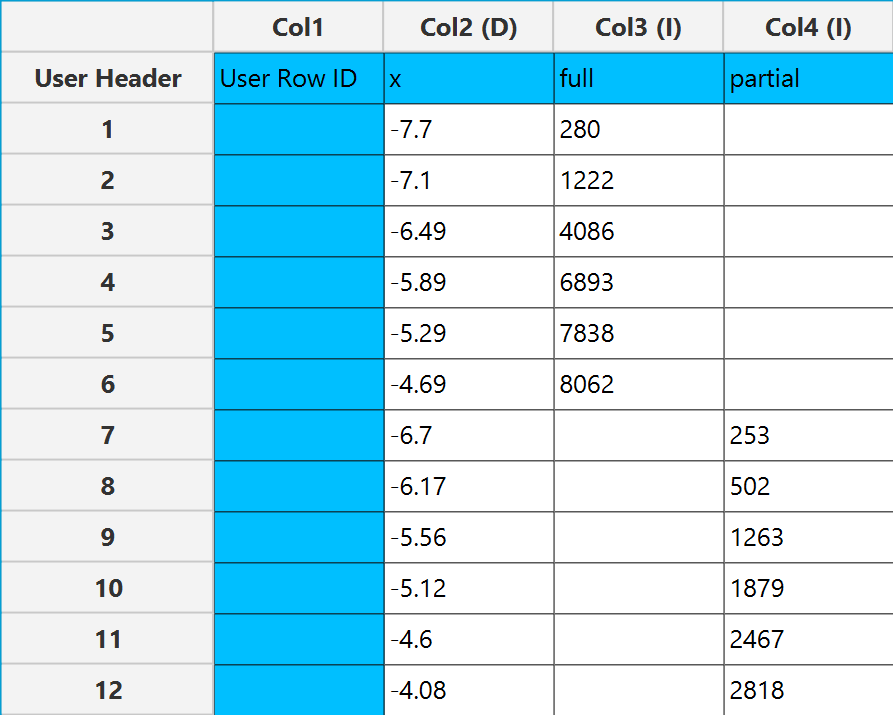
In the input datasheet the requirement is to specify at least two numerical columns and insert the appropriate data, as shown below.

Configuration

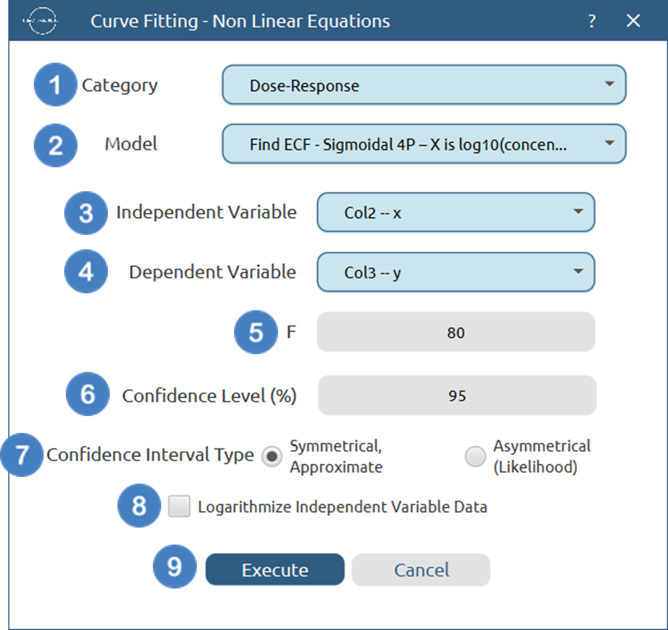
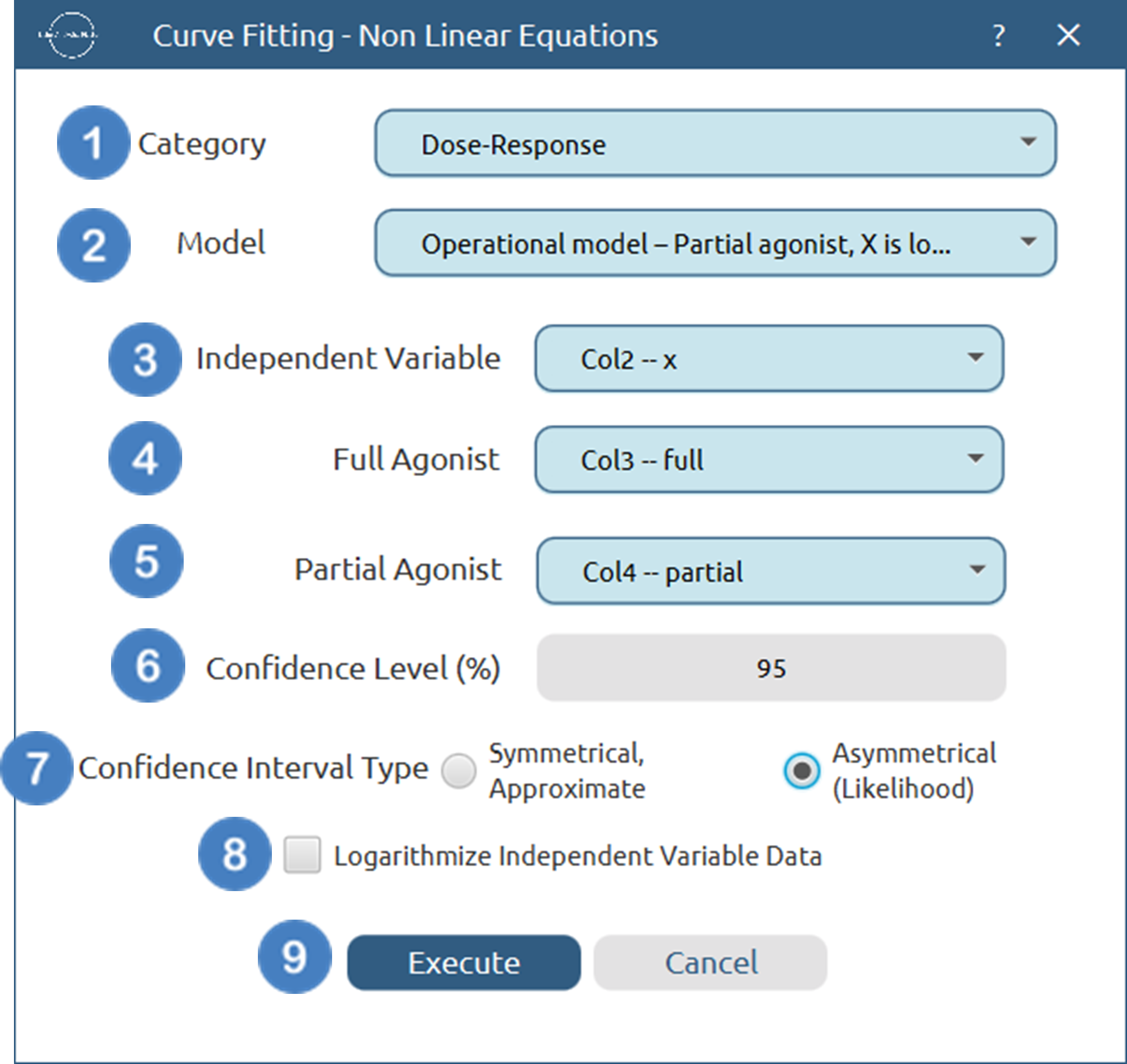
1. Select Statistics → Curve Fitting → Non Linear Equations.
2. Specify the Category [1] of the model you wish to use.
3. Select the specific Model [2] to fit.
4. Select the column that corresponds to the Independent Variable[3].
5. Select the column that corresponds to the Dependent Variable[4].
6. Specify the value of any extra parameters for the specified model [5].
7. Specify the Confidence Level (%)[6] for tests.
8. Select the Confidence Interval Type [7].
9. Select/tick if you wish to Logarithmize Independent Variable Data before fitting [8].
10. Click on the Execute button [9] to perform the Non Linear Curve Fitting method.

Output

The parameter estimates and goodness of fit tables are shown in the output spreadsheet and the line chart showcasing the fitted curve and the experimental points is shown in a separate window.

Case 2: Two dependent variables

Input

Numerical values should be specified in the input datasheet. The design Non Linear Equations with two dependent variable (Case 2) requires at least three columns in the input sheet: one column representing the independent variable, and two columns for the numerical responses variable (dependent variables). The independent-variable column must not contain empty cells. Missing values are allowed only in the dependent-variable columns; rows with missing Y values are excluded from the fit for that specific dependent variable. Each row corresponds to a single observation.

Configuration

Category	Select the model family that best matches your analysis.
Model	Select the specific equation to fit within the chosen category.
Independent Variable	Select the column that corresponds to values of the independent variable.
Dependent Variables	Select the column that corresponds to values of each dependent variable. For each specific model that requires two dependent variables the label is changed to describe what the algorithm expects for each dependent variable.
Extra Parameters	Enter values for any additional model-specific parameters required for the selected equation. Refer to the documentation for the chosen model (in the list of available models) for the definition, allowed range/options, and recommended settings for each extra parameter.
Confidence Level (%)	Specify the confidence level of the analysis. Values should range from 0 to 100 and correspond to percentages.
Confidence Interval Type	Choose how confidence intervals are computed: Symmetrical, Approximate and Assymetrical(Likelihood).
Logarithmize Independent Variable Data	Use this option to logarithmize (base 10) the data in the specified independent variable column.

Output

The output spreadsheet contains two tables:

1. Parameter Estimates: Reports the fitted value for each estimated parameter along with the lower and upper confidence limits at the selected confidence level. For parameters expressed on a log scale (e.g., LogEC50), the output also includes the corresponding back-transformed values (e.g., EC50) and their confidence limits.
2. Goodness of Fit: Summarizes overall fit statistics, including the number of data points used, degrees of freedom, residual sum of squares (SS), and the standard error of the regression.

In addition, a pop-up window displays a plot of the fitted curve overlaid with the experimental data points for each dependent variable.

Example

Input

In the input datasheet the requirement is to specify at least three numerical columns and insert the appropriate data, as shown below.

Configuration

1. Select Statistics → Curve Fitting → Non Linear Equations.
2. Specify the Category [1] of the model you wish to use.
3. Select the specific Model [2] to fit.
4. Select the column that corresponds to the Independent Variable[3].
5. Select the column that corresponds to the two Dependent Variables[4], [5].
6. Specify the Confidence Level (%)[6] for tests.
7. Select the Confidence Interval Type [7].
8. Select/tick if you wish to Logarithmize Independent Variable Data before fitting [8].
9. Click on the Execute button [9] to perform the Non Linear Curve Fitting method.

Output

The parameter estimates and goodness of fit tables are shown in the output spreadsheet and the line chart showcasing the fitted curve and the experimental points for each dependent variable is shown in a separate window.

Case 3: Multi-dependent variable models

Input

Numerical values should be specified in the input datasheet. The design Non Linear Equations with multiple dependent variables (Case 3) requires at least three columns in the input sheet: one column representing the independent variable, and at least two columns for the numerical responses variable (dependent variables). The independent-variable column must not contain empty cells. Missing values are allowed only in the dependent-variable columns; rows with missing Y values are excluded from the fit for that specific dependent variable. Each row corresponds to a single observation.

Configuration

Category	Select the model family that best matches your analysis.
Model	Select the specific equation to fit within the chosen category.
Add Column Pair(s)	Click to open the dialog for adding independent–dependent variable column pairs.
Select X Column/ Select Y Column/Concentration Value	Choose the column for the independent variable (X) and the column for the dependent variable (Y), and enter the corresponding ligand concentration for that pair.
Add/Add & Close/Close	Use these buttons to add the specified pair, add and close the dialog, or close without adding.
Remove Selected Column Pair(s)	Remove the currently selected column pair(s).
Extra Parameters	Enter values for any additional model-specific parameters required for the selected equation. Refer to the documentation for the chosen model (in the list of available models) for the definition, allowed range/options, and recommended settings for each extra parameter.
Confidence Level (%)	Specify the confidence level of the analysis. Values should range from 0 to 100 and correspond to percentages.
Confidence Interval Type	Choose how confidence intervals are computed: Symmetrical, Approximate and Assymetrical(Likelihood).
Logarithmize Independent Variable Data	Use this option to logarithmize (base 10) the data in the specified independent variable column.

Output

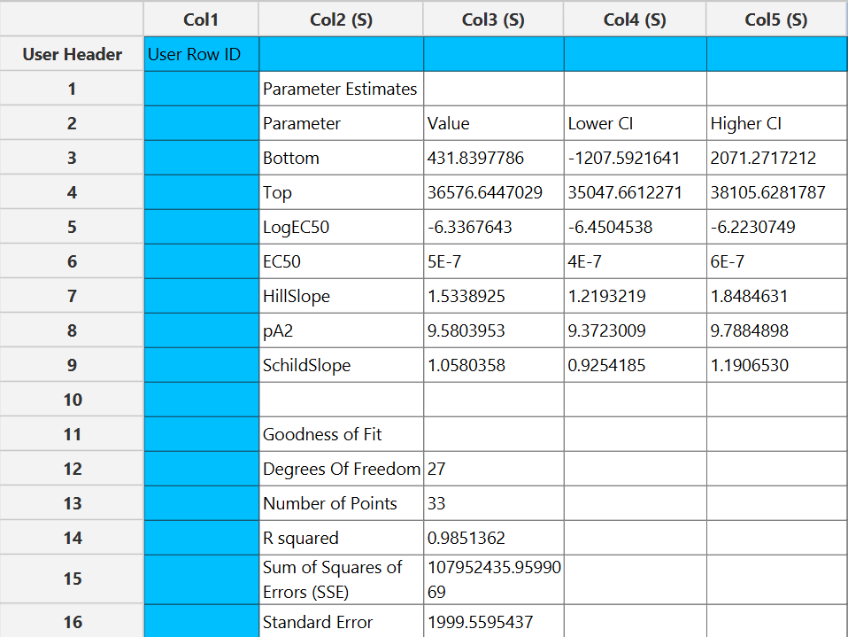
The output spreadsheet contains two tables:

1. Parameter Estimates: Reports the fitted value for each estimated parameter along with the lower and upper confidence limits at the selected confidence level. For parameters expressed on a log scale (e.g., LogEC50), the output also includes the corresponding back-transformed values (e.g., EC50) and their confidence limits.
2. Goodness of Fit: Summarizes overall fit statistics, including the number of data points used, degrees of freedom, residual sum of squares (SS), and the standard error of the regression.

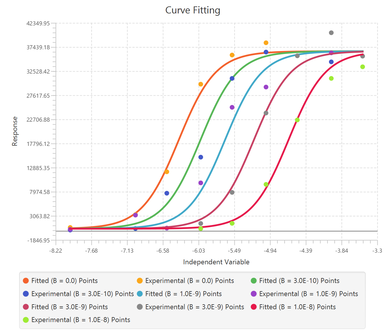
In addition, a pop-up window displays a plot of the fitted curve overlaid with the experimental data points for each dependent variable.

Example

Input

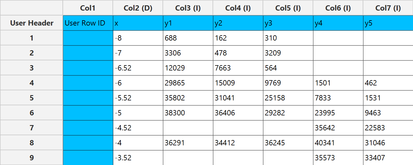
In the input datasheet the requirement is to specify at least three numerical columns and insert the appropriate data, as shown below.

Configuration

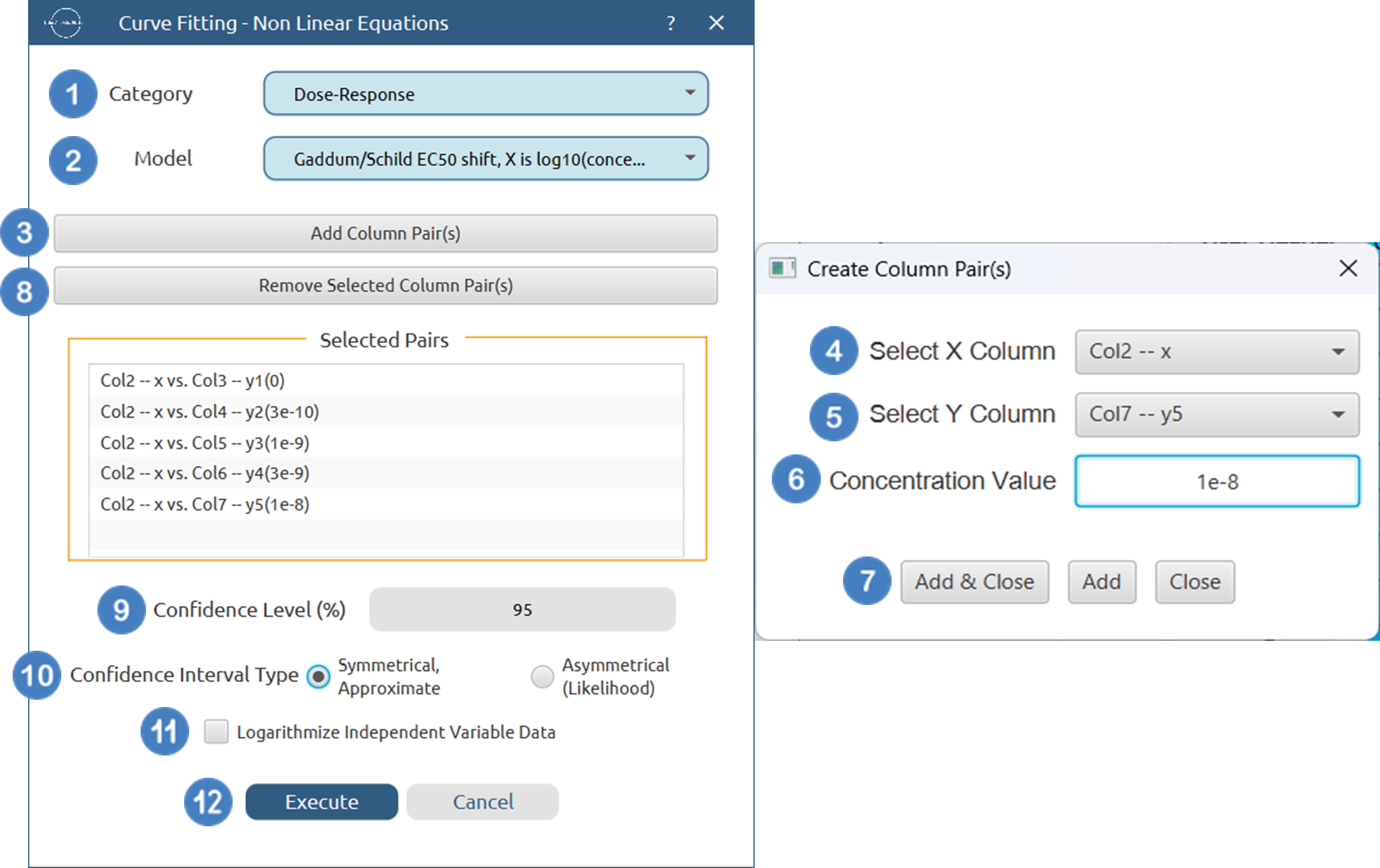
1. Select Statistics → Curve Fitting → Non Linear Equations.
2. Specify the Category [1] of the model you wish to use.
3. Select the specific Model [2] to fit.
4. Click on the Add Column Pair(s)[3] button to open the column pairs dialogue.
5. Select the column that corresponds to the independent variable (X Column) [4], the column that corresponds to the dependent variable (Y Column) [5] and specify the Concentration Value[6] of the ligand for each pair. Use these buttons at the bottom of the dialogue[7] to add the specified pair, add and close the dialog, or close without adding.
6. Optionally Remove Selected Column Pair(s)[8] that are not wanted in the analysis.
7. Specify the Confidence Level (%)[9] for tests.
8. Select the Confidence Interval Type [10].
9. Select/tick if you wish to Logarithmize Independent Variable Data before fitting [11].
10. Click on the Execute button [12] to perform the Non Linear Curve Fitting method.

Output

The parameter estimates and goodness of fit tables are shown in the output spreadsheet and the line chart showcasing the fitted curve and the experimental points for each dependent variable is shown in a separate window.

---

Available Models

Dose-Response

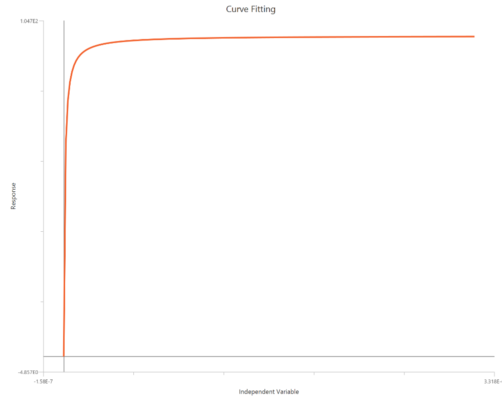
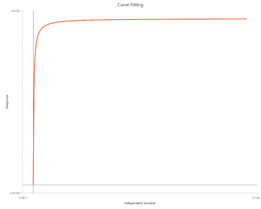
Inhibitor – Sigmoidal 4P – Raw response

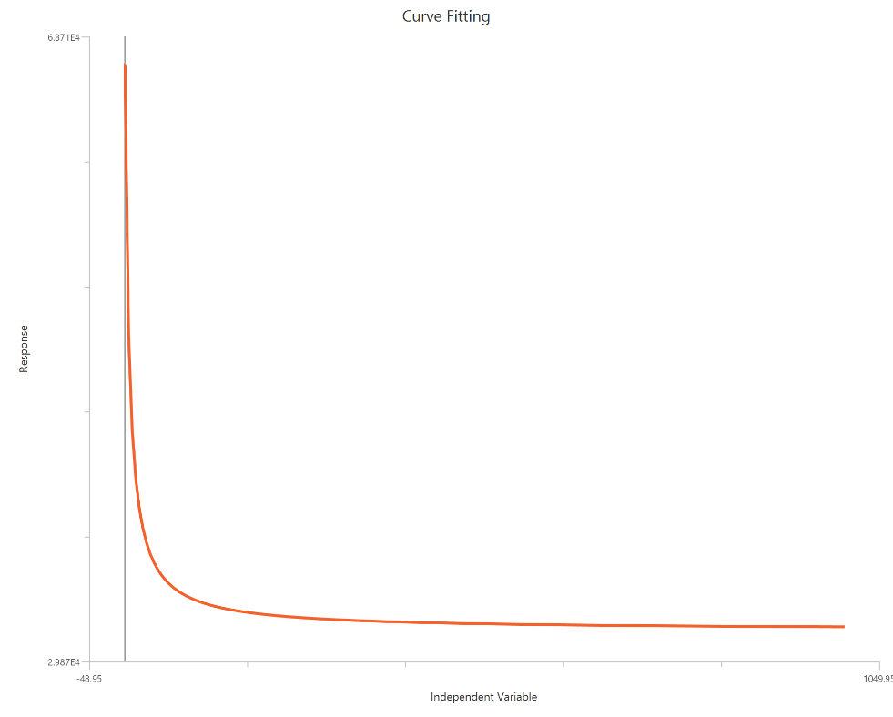
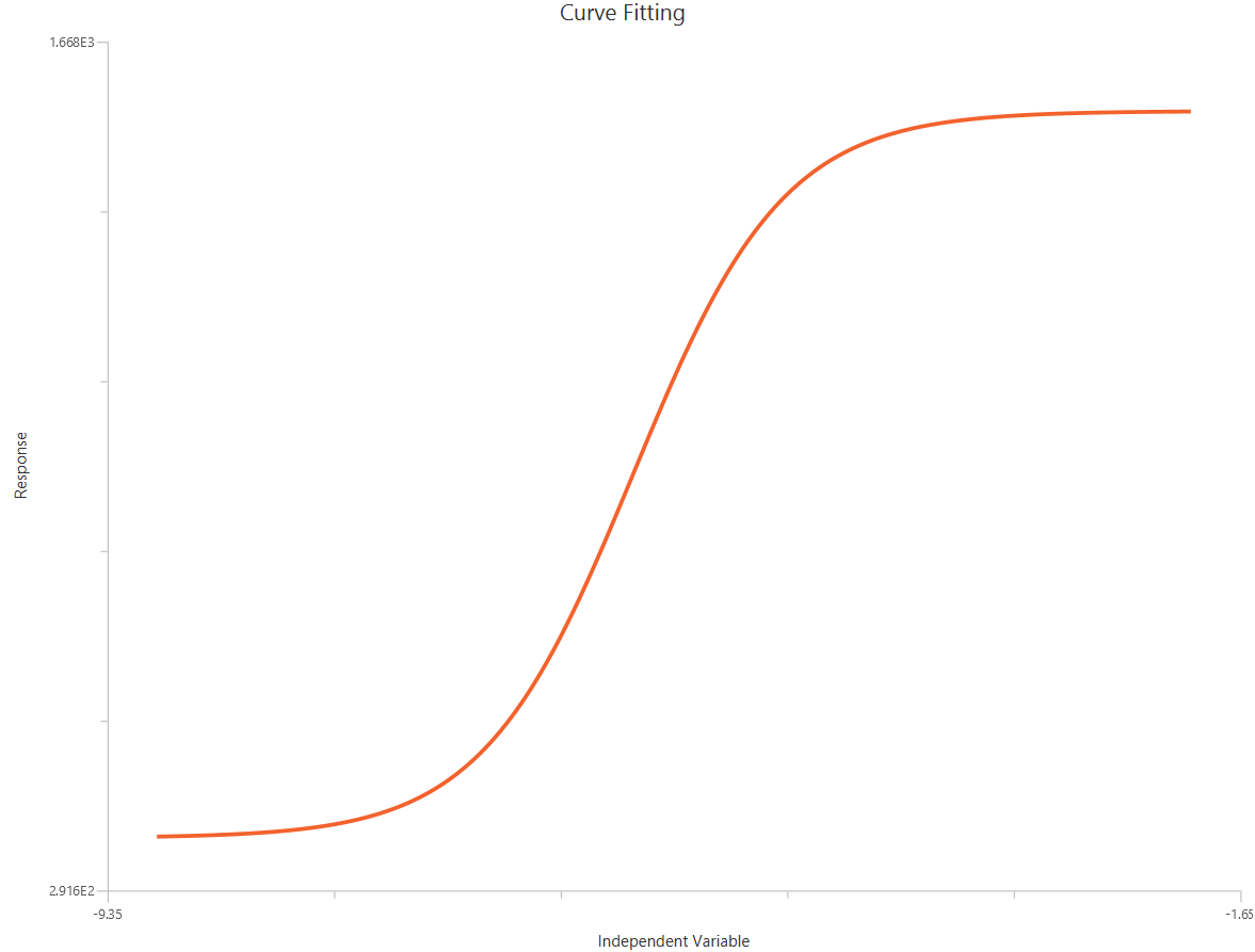
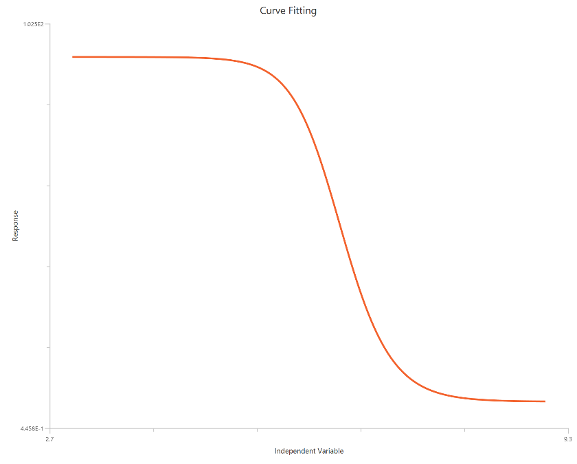
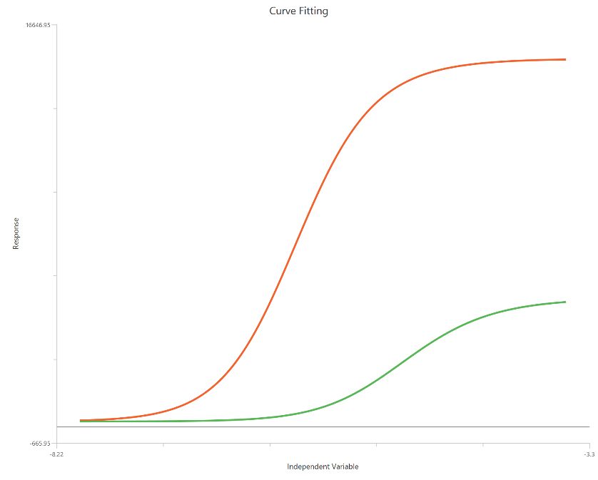
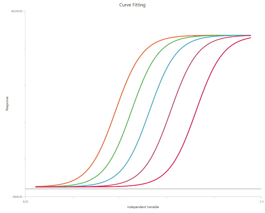
The Inhibitor – Sigmoidal 4P – Raw response model fits a monophasic inhibitory Hill-type sigmoidal curve using linear inhibitor concentration on the X-axis. It estimates Top (uninhibited plateau), Bottom (maximally inhibited plateau), the IC50 (inhibitor concentration producing 50% inhibition across the response range), and a free HillSlope that controls curve steepness/apparent cooperativity. Because the X-axis is linear, the low-concentration region is compressed, so dense sampling around IC50 is important to define the transition reliably. This 4-parameter form is preferred when both asymptotes are supported by the data and slope differences are biologically or experimentally relevant.

Equation

\begin{equation} \begin{alignedat}{1} Y &= \mathrm{Bottom} + \frac{\mathrm{Top} - \mathrm{Bottom}}{1 + (\frac{\mathrm{IC50}}{X})^{\mathrm{HillSlope}}} \end{alignedat} \end{equation}

Visualization

Input

The independent variable (X) must be the concentration/dose on a linear scale and therefore must be strictly positive \((X>0)\). Zero or negative X values are not used in the calculations (they are ignored/excluded). The model also requires a column containing the dependent variable (Y) response values (in any consistent units).

Parameters

1. \(Top:\) The upper asymptote (response with ~0 inhibitor), representing the uninhibited control plateau.

2. \(Bottom\): The lower asymptote at high inhibitor, representing the maximally inhibited plateau (residual activity/background).

3. \(IC50\): The inhibitor concentration that reduces the response by 50% over the dynamic range between the Top (uninhibited) and Bottom (maximally inhibited) plateaus; it is a standard measure of inhibitory potency. Lower IC50 indicates higher potency under the same assay conditions.

4. \(HillSlope\): The slope factor controlling the steepness of the inhibitory transition; reflects apparent cooperativity/heterogeneity (not necessarily mechanistic).

---

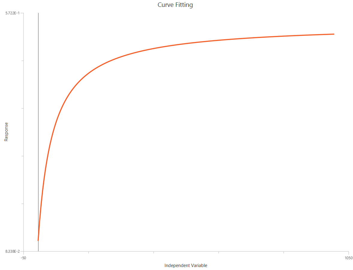
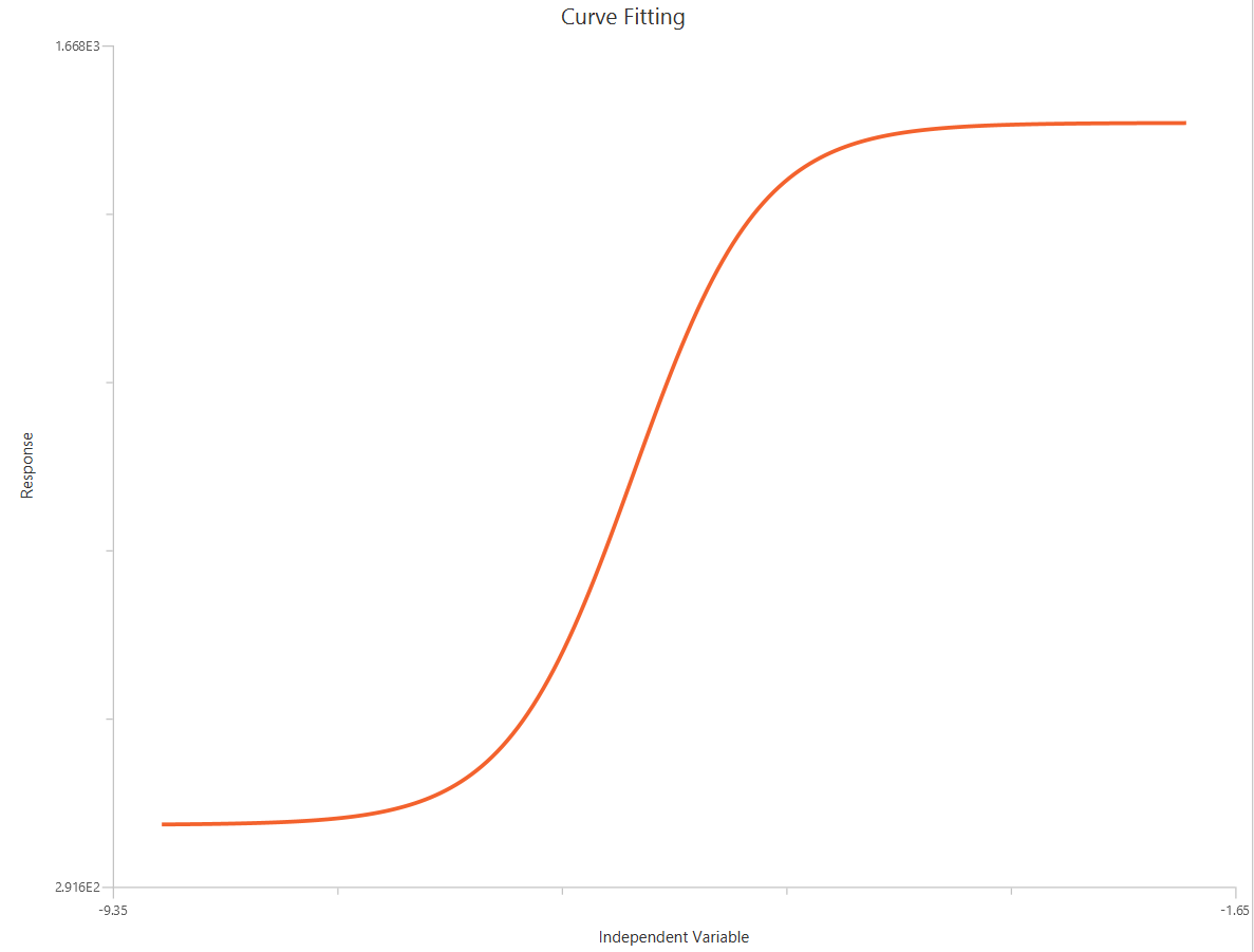
Inhibitor – Sigmoidal 3P (slope = 1) – Raw response

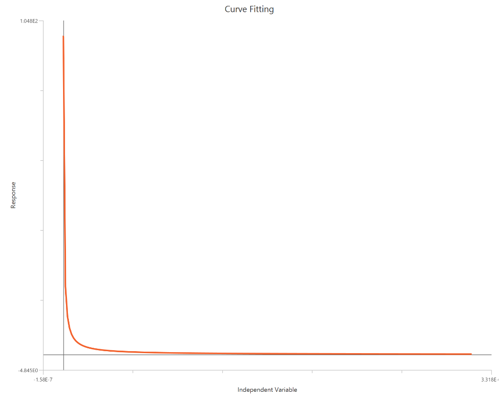
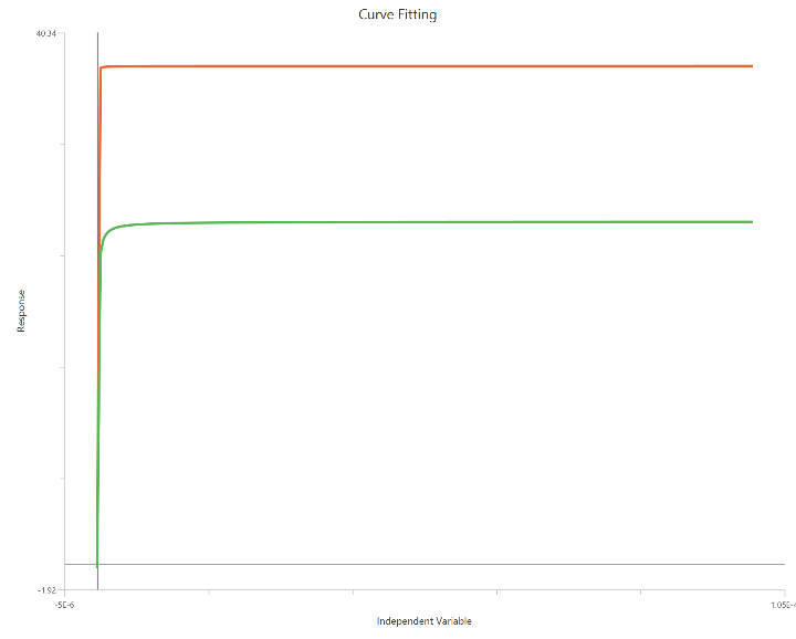
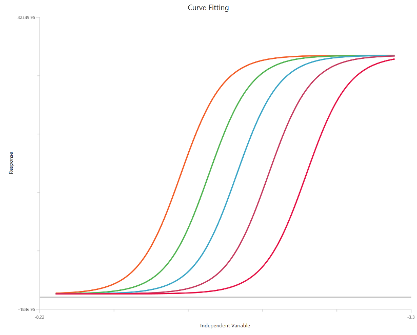
The Inhibitor – Sigmoidal 3P (slope = 1) – Raw response model fits a monophasic inhibitory sigmoidal relationship using linear inhibitor concentration on the X-axis. In this formulation the HillSlope is fixed to 1, imposing a standard steepness and reducing model flexibility. The fit focuses on estimating IC50 (potency, in concentration units) and the two free plateau. Because the X-axis is linear, dense sampling around IC50 is important to define the transition accurately.

Equation

\begin{equation} \begin{alignedat}{1} Y &= \mathrm{Bottom} + \frac{\mathrm{Top} - \mathrm{Bottom}}{1 + \frac{X}{IC50}} \end{alignedat} \end{equation}

Visualization

Input

The independent variable (X) must be the concentration/dose on a linear scale and therefore must be strictly positive \((X>0)\). Zero or negative X values are not used in the calculations (they are ignored/excluded). The model also requires a column containing the dependent variable (Y) response values (in any consistent units).

Parameters

1. \(Top:\) The upper asymptote (response with ~0 inhibitor), representing the uninhibited control plateau.

2. \(Bottom\): The lower asymptote at high inhibitor, representing the maximally inhibited plateau (residual activity/background).

3. \(IC50\): The inhibitor concentration that reduces the response by 50% over the dynamic range between the Top (uninhibited) and Bottom (maximally inhibited) plateaus; it is a standard measure of inhibitory potency. Lower IC50 indicates higher potency under the same assay conditions.

---

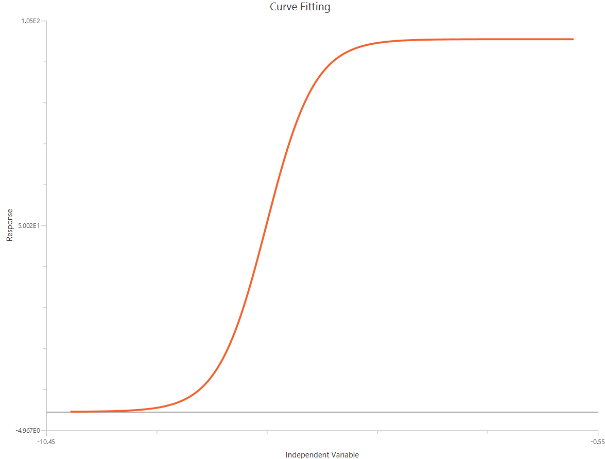
Inhibitor – Sigmoidal 4P – Normalized 0–100% response

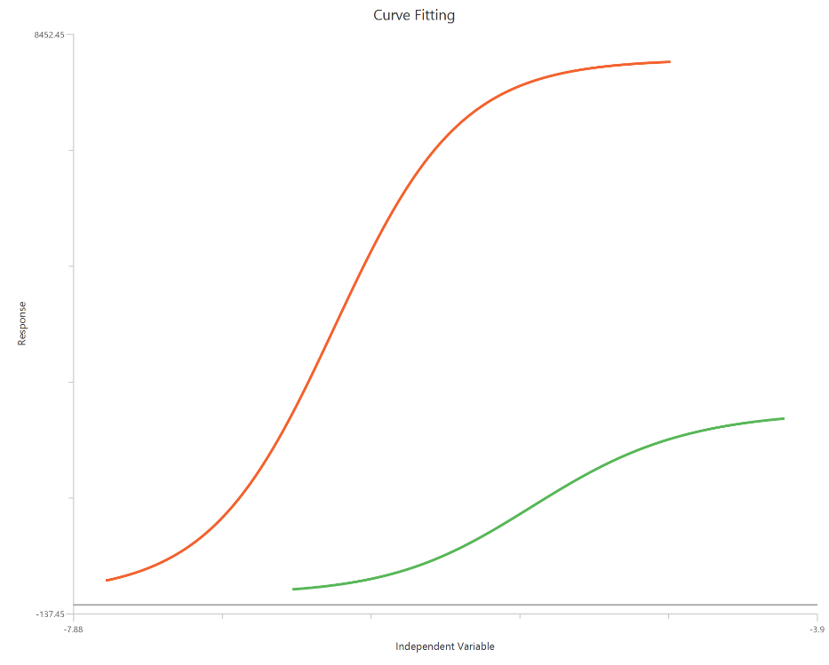
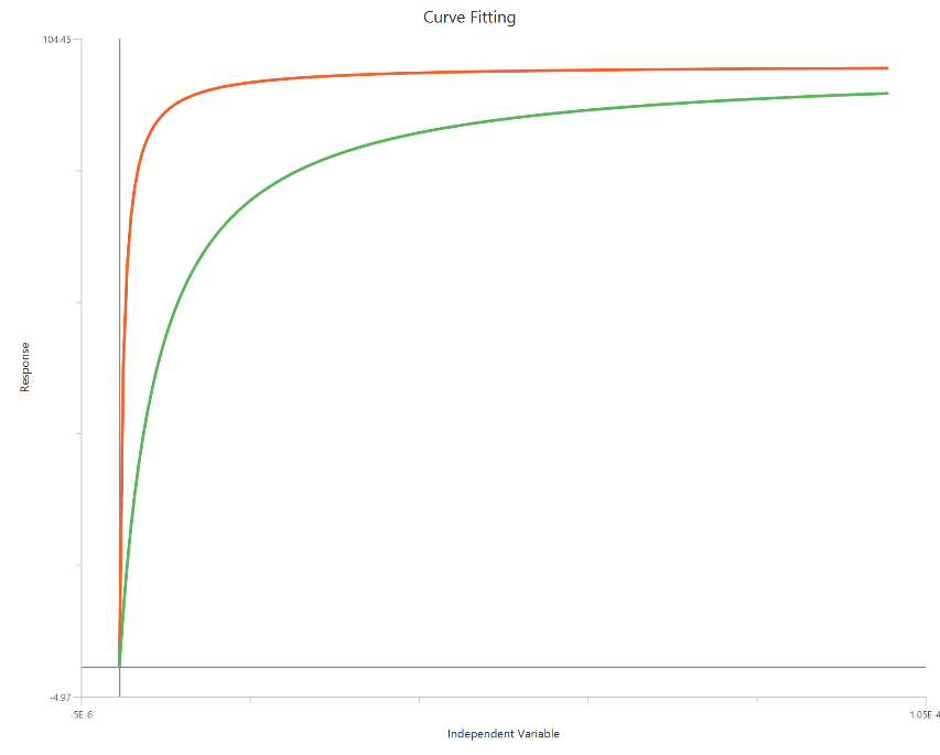
The Inhibitor – Sigmoidal 4P – Normalized 0–100% response model fits a monophasic inhibitory sigmoidal curve to normalized data (e.g., % of control) using linear inhibitor concentration on the X-axis. Normalization constrains the response range to 100% (Top) at low inhibitor and 0% (Bottom) at high inhibitor, improving comparability across experiments. The fit estimates IC50 (in concentration units) and a free HillSlope that governs steepness/apparent cooperativity, while Top/Bottom may be fixed or constrained depending on the normalization. Because the X-axis is linear, dense sampling around IC50 is important for robust potency and slope estimates.

Equation

\begin{equation} \begin{alignedat}{1} Y &= \frac{100}{1 + (\frac{\mathrm{IC50}}{X})^{\mathrm{HillSlope}}} \end{alignedat} \end{equation}

Visualization

Input

The independent variable (X) must be the concentration/dose on a linear scale and therefore must be strictly positive \((X>0)\). Zero or negative X values are not used in the calculations (they are ignored/excluded). The model also requires a column containing the dependent variable (Y) response values (in any consistent units).

Parameters

1. \(IC50\): The inhibitor concentration that reduces the response by 50% over the dynamic range between the Top (uninhibited) and Bottom (maximally inhibited) plateaus; it is a standard measure of inhibitory potency. Lower IC50 indicates higher potency under the same assay conditions.

2. \(HillSlope\): The slope factor controlling the steepness of the inhibitory transition; reflects apparent cooperativity/heterogeneity (not necessarily mechanistic).

---

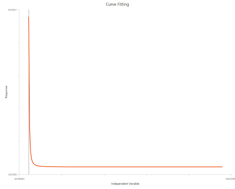
Inhibitor – Sigmoidal 3P (slope = 1) – Normalized 0–100% response

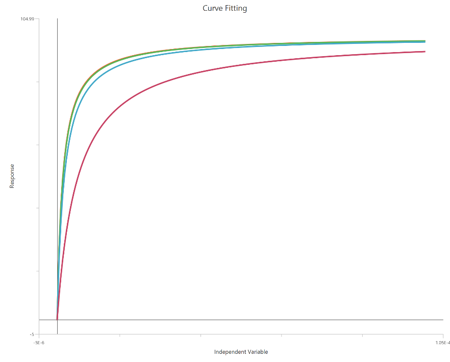
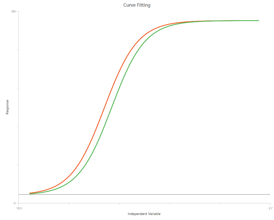
The Inhibitor – Sigmoidal 3P (slope = 1) – Normalized 0–100% response model fits a monophasic inhibitory sigmoidal relationship to data normalized to % of control (or similar) using linear inhibitor concentration on the X-axis. In this formulation the HillSlope is fixed to 1, imposing a standard steepness and focusing interpretation on potency shifts. Normalization constrains the response range near 100% (Top) at low inhibitor and 0% (Bottom) at high inhibitor, with Top/Bottom fixed to 100/0. The fit primarily estimates IC50 (in concentration units), so adequate sampling around IC50 is critical given the compressed low-dose region on a linear X-axis.

Equation

\begin{equation} \begin{alignedat}{1} Y &= \frac{100}{1 + \frac{X}{\mathrm{IC50}}} \end{alignedat} \end{equation}

Visualization

Input

The independent variable (X) must be the concentration/dose on a linear scale and therefore must be strictly positive \((X>0)\). Zero or negative X values are not used in the calculations (they are ignored/excluded). The model also requires a column containing the dependent variable (Y) response values (in any consistent units).

Parameters

1. \(IC50\): The inhibitor concentration that reduces the response by 50% over the dynamic range between the Top (uninhibited) and Bottom (maximally inhibited) plateaus; it is a standard measure of inhibitory potency. Lower IC50 indicates higher potency under the same assay conditions.

---

log10(Inhibitor) – Sigmoidal 4P – Raw response

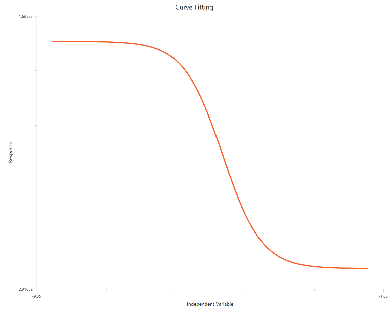
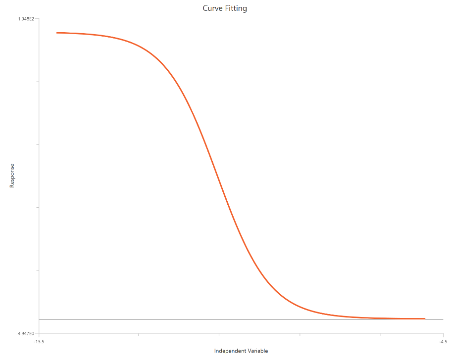
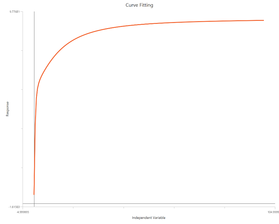
The log10(Inhibitor) – Sigmoidal 4P – Raw response model fits a monophasic inhibitory sigmoidal curve with \(X = log_{10}(inhibitor)\). It estimates the Top (uninhibited plateau) and Bottom (maximally inhibited plateau), the logIC50 (log10 inhibitor concentration giving 50% inhibition across the response range), and a free HillSlope that controls curve steepness/apparent cooperativity. The log-scaled X-axis spreads the low-dose region, improving definition of the transition around IC50.

Equation

\begin{equation} \begin{alignedat}{1} Y &= \mathrm{Bottom} + \frac{\mathrm{Top} - \mathrm{Bottom}}{1 + 10^{(\mathrm{LogIC50} - X) \cdot \mathrm{HillSlope}}} \end{alignedat} \end{equation}

Visualization

Input

The independent variable (X) must be the log10-transformed concentration/dose (i.e., \(𝑋 = log_{10}(concentration/dose)\)). The model also requires a column containing the dependent variable (Y) response values (in any consistent units).

Parameters

1. \(Top:\) The upper asymptote (response with ~0 inhibitor), representing the uninhibited control plateau.

2. \(Bottom\): The lower asymptote at high inhibitor, representing the maximally inhibited plateau (residual activity/background).

3. \(LogIC50\): The log10 inhibitor concentration that produces 50% inhibition of the response range between Top and Bottom; a measure of inhibitory potency.

4. \(HillSlope\): The slope factor controlling the steepness of the inhibitory transition; reflects apparent cooperativity/heterogeneity (not necessarily mechanistic).

---

log10(Inhibitor) – Sigmoidal 3P (slope = 1) – Raw response

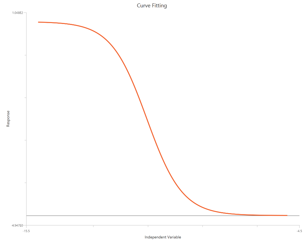
The log(inhibitor) vs. response (three parameters) model describes a monophasic inhibitory sigmoidal dose–response relationship with \(X = log_{10}(inhibitor)\). It is a reduced form of the 4PL where one \(HillSlope = 1\). This constraint improves fit stability when the data do not adequately define both asymptotes.

Equation

\begin{equation} \begin{alignedat}{1} Y &= \mathrm{Bottom} + \frac{\mathrm{Top} - \mathrm{Bottom}}{1 + 10^{(X - \mathrm{LogIC50})}} \end{alignedat} \end{equation}

Visualization

Input

The independent variable (X) must be the log10-transformed concentration/dose (i.e., \(𝑋 = log_{10}(concentration/dose)\)). The model also requires a column containing the dependent variable (Y) response values (in any consistent units).

Parameters

1. \(Top:\) The upper asymptote (response with ~0 inhibitor), representing the uninhibited control plateau.

2. \(Bottom\): The lower asymptote at high inhibitor, representing the maximally inhibited plateau (residual activity/background).

3. \(LogIC50\): The log10 inhibitor concentration that produces 50% inhibition of the response range between Top and Bottom; a measure of inhibitory potency.

---

log10(Inhibitor) – Sigmoidal 4P – Normalized 0–100% response

The log(inhibitor) vs. normalized response — variable slope model fits a monophasic inhibitory sigmoidal curve to normalized data (e.g., % of control) using \(X = log_{10}(inhibitor)\). Normalization constrains the response range near 100% (Top) and 0% (Bottom), while the fit estimates logIC50 (inhibitory potency) and a free HillSlope that governs steepness/apparent cooperativity. The log-scaled X-axis expands the low-dose region, improving definition of the transition around IC50. This formulation is preferred for comparing potency and slope across conditions when absolute signal amplitudes differ between experiments. Bottom and Top are fixed to 0 and 100 respectively.

Equation

\begin{equation} \begin{alignedat}{1} Y &= \frac{100}{1 + 10^{(\mathrm{LogIC50} - X) \cdot \mathrm{HillSlope}}} \end{alignedat} \end{equation}

Visualization

Input

The independent variable (X) must be the log10-transformed concentration/dose (i.e., \(𝑋 = log_{10}(concentration/dose)\)). The model also requires a column containing the dependent variable (Y) response values (in any consistent units).

Parameters

1. \(LogIC50\): The log10 inhibitor concentration that produces 50% inhibition of the response range between Top and Bottom; a measure of inhibitory potency.

2. \(HillSlope\): The slope factor controlling the steepness of the inhibitory transition; reflects apparent cooperativity/heterogeneity (not necessarily mechanistic).

---

log10(Inhibitor) – Sigmoidal 3P (slope = 1) – Normalized 0–100% response

The log(inhibitor) vs. normalized response model fits a monophasic inhibitory sigmoidal relationship to responses normalized to % of control (or similar), with \(X = log10[inhibitor]\). Normalization constrains the response scale so the curve spans from ~100% (Top) at low inhibitor to ~0% (Bottom) at high inhibitor, improving comparability across runs. The fit is used to estimate logIC50 (inhibitory potency). Bottom and Top are fixed to 0 and 100 respectively and Hillslope is fixed to 1.

Equation

\begin{equation} \begin{alignedat}{1} Y &= \frac{100}{1 + 10^{(X - \mathrm{LogIC50})}} \end{alignedat} \end{equation}

Visualization

Input

The independent variable (X) must be the log10-transformed concentration/dose (i.e., \(𝑋 = log_{10}(concentration/dose)\)). The model also requires a column containing the dependent variable (Y) response values (in any consistent units).

Parameters

1. \(LogIC50\): The log10 inhibitor concentration that produces 50% inhibition of the response range between Top and Bottom; a measure of inhibitory potency.

---

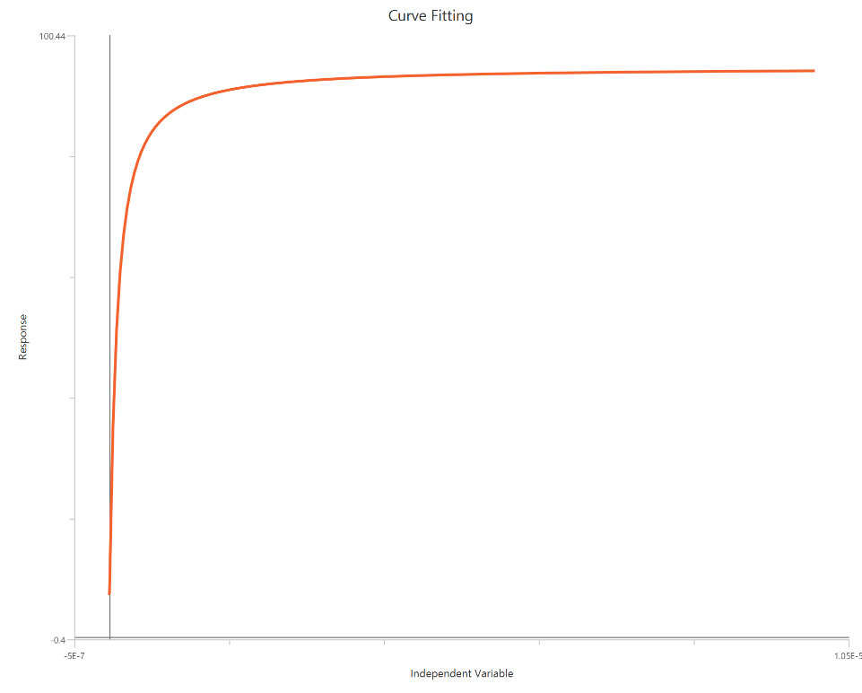
Agonist – Sigmoidal 4P – Raw response

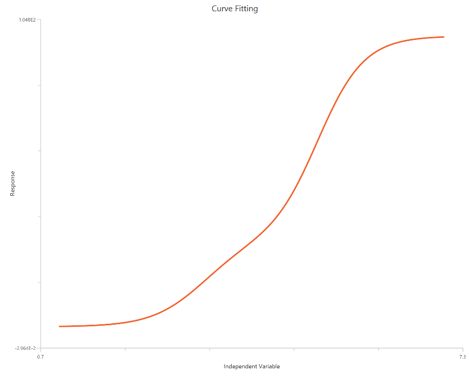
The Agonist – Sigmoidal 4P – Raw response model describes a monophasic Hill-type sigmoidal concentration–response curve using the linear agonist concentration on the X-axis. It estimates Bottom and Top plateaus, the EC50 (potency, in concentration units), and a free HillSlope that governs curve steepness/apparent cooperativity. Unlike log-transformed X models, linear scaling compresses the low-concentration region, so dense sampling around the EC50 is critical for stable parameter estimation. This 4-parameter form is preferred when both baseline and maximal plateaus are experimentally defined and should be fit rather than constrained.

Equation

\[ \begin{equation} \begin{alignedat}{1} Y &= \mathrm{Bottom} + \frac{(X^{\mathrm{HillSlope}}) \cdot (\mathrm{Top} - \mathrm{Bottom})}{(X^{\mathrm{HillSlope}} + \mathrm{EC50}^{\mathrm{HillSlope}})} \end{alignedat} \end{equation} \]

Visualization

Input

The independent variable (X) must be the concentration/dose on a linear scale and therefore must be strictly positive \((X>0)\). Zero or negative X values are not used in the calculations (they are ignored/excluded). The model also requires a column containing the dependent variable (Y) response values (in any consistent units).

Parameters

1. \(Bottom\): The lower asymptote of the curve (minimal response at very low agonist), often representing baseline activity/background.

2. \(Top\): The upper asymptote (maximal response at saturating agonist), i.e., the observed Emax plateau.

3. \(HillSlope\): The slope factor that determines the steepness of the sigmoidal transition; reflects apparent cooperativity (not necessarily).

4. \(EC50\): The agonist concentration that produces 50% of the maximal effect (halfway between Bottom and Top), and is a standard measure of potency. Lower EC50 indicates higher potency under the same assay conditions.

---

Agonist – Sigmoidal 3P (slope = 1) – Raw response

The Agonist – Sigmoidal 3P (slope = 1) – Raw response model fits a Hill-type sigmoidal relationship using the linear agonist concentration on the X-axis (not log-transformed). It is a reduced form where HillSlope is fixed to 1. The remaining parameters estimate EC50 (potency, in concentration units), Top and Bottom. Because the X-axis is linear, low-dose regions are less “spread out,” so good sampling near EC50 is especially important for reliable fits.

Equation

\[ \begin{equation} \begin{alignedat}{1} Y &= \mathrm{Bottom} + X \cdot \frac{\mathrm{Top} - \mathrm{Bottom}}{\mathrm{EC50} + X} \end{alignedat} \end{equation} \]

Visualization

Input

The independent variable (X) must be the concentration/dose on a linear scale and therefore must be strictly positive \((X>0)\). Zero or negative X values are not used in the calculations (they are ignored/excluded). The model also requires a column containing the dependent variable (Y) response values (in any consistent units).

Parameters

1. \(Bottom\): The lower asymptote of the curve (minimal response at very low agonist), often representing baseline activity/background.

2. \(Top\): The upper asymptote (maximal response at saturating agonist), i.e., the observed Emax plateau.

3. \(EC50\): The agonist concentration that produces 50% of the maximal effect (halfway between Bottom and Top), and is a standard measure of potency. Lower EC50 indicates higher potency under the same assay conditions.

---

Agonist – Sigmoidal 4P – Normalized 0–100% response

The Agonist – Sigmoidal 4P – Normalized 0–100% response model fits a Hill-type sigmoidal concentration–response curve to normalized data (e.g., % of control or % maximal) using linear agonist concentration on the X-axis. Normalization constrains the response range near 0% (Bottom) and 100% (Top), while the fit estimates EC50 (potency) and a free HillSlope that sets the curve steepness/apparent cooperativity. Because the X-axis is not log-transformed, the low-dose region is compressed, so dense measurements near EC50 are important for robust slope and potency estimates. This model is well suited for comparing potency and slope across conditions when absolute signal amplitudes vary between runs.

Equation

\[ \begin{equation} \begin{alignedat}{1} Y &= \frac{100 \cdot (X^{\mathrm{HillSlope}})}{EC50^{\mathrm{HillSlope}} + X^{\mathrm{HillSlope}}} \end{alignedat} \end{equation} \]

Visualization

Input

The independent variable (X) must be the concentration/dose on a linear scale and therefore must be strictly positive \((X>0)\). Zero or negative X values are not used in the calculations (they are ignored/excluded). The model also requires a column containing the dependent variable (Y) response values (in any consistent units).

Parameters

1. \(EC50\): The agonist concentration that produces 50% of the maximal effect (halfway between Bottom and Top), and is a standard measure of potency. Lower EC50 indicates higher potency under the same assay conditions.

2. \(HillSlope\): The slope factor that determines the steepness of the sigmoidal transition; reflects apparent cooperativity (not necessarily).

---

Agonist – Sigmoidal 3P (slope = 1) – Normalized 0–100% response

The Agonist – Sigmoidal 3P (slope = 1) – Normalized 0–100% response model fits a Hill-type sigmoidal concentration–response relationship to data normalized to % of control or % of maximal response, using linear agonist concentration on the X-axis. Normalization constrains the response scale so the asymptotes are at 0% (Bottom) and 100% (Top), improving comparability across experiments. The fit is used to estimate EC50 (potency, in concentration units) while the HillSlope (steepness/apparent cooperativity) is fixed to 1 and Bottom/Top are fixed to 0 and 100 respectively. Because the X-axis is linear, adequate sampling around EC50 is especially important to define the transition region accurately.

Equation

\[ \begin{equation} \begin{alignedat}{1} Y &= \frac{100 \cdot X}{\mathrm{EC50} + x} \end{alignedat} \end{equation} \]

Visualization

Input

The independent variable (X) must be the concentration/dose on a linear scale and therefore must be strictly positive \((X>0)\). Zero or negative X values are not used in the calculations (they are ignored/excluded). The model also requires a column containing the dependent variable (Y) response values (in any consistent units).

Parameters

1. \(EC50\): The agonist concentration that produces 50% of the maximal effect (halfway between Bottom and Top), and is a standard measure of potency. Lower EC50 indicates higher potency under the same assay conditions.

---

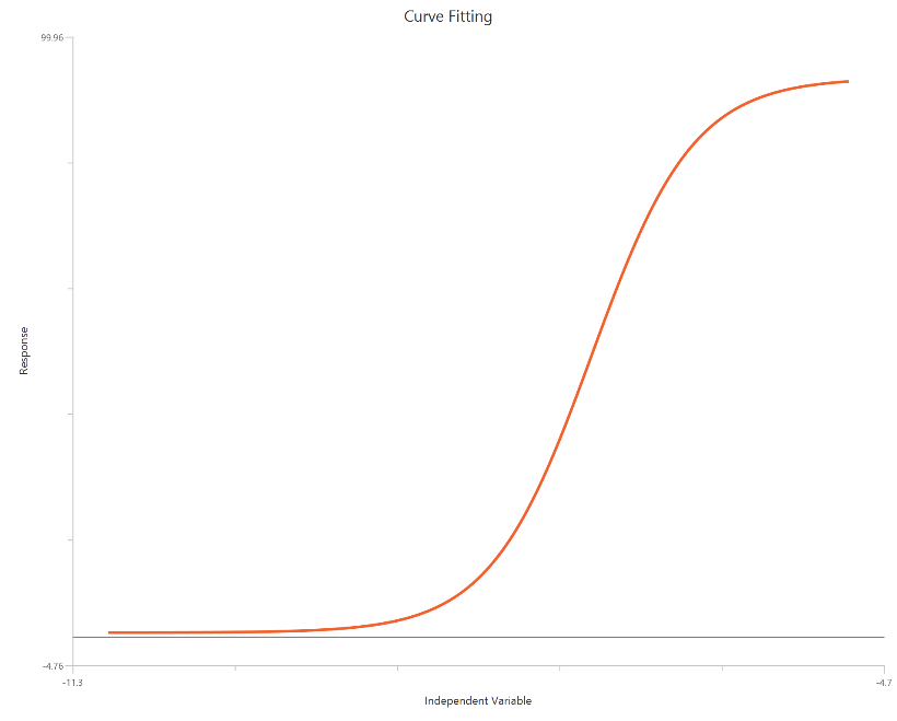
log10(Agonist) – Sigmoidal 4P – Raw response

The log10(Agonist) – Sigmoidal 4P – Raw response model describes a monophasic sigmoidal concentration–response relationship with \(X=log_{10}(agonist)\). The curve is parameterized by Bottom and Top plateaus, logEC50 (the log concentration producing 50% of the maximal effect), and the Hill slope. Allowing a variable Hill slope captures differences in steepness/cooperativity rather than assuming a fixed unit slope. It is the standard choice for estimating potency (EC50) and efficacy (Emax/Top) when no biphasic behavior is present.

Equation

\[ \begin{equation} \begin{alignedat}{1} Y &= \mathrm{Bottom} + \frac{\mathrm{Top} - \mathrm{Bottom}}{1 + 10^{(\mathrm{LogEC50} - X) \cdot \mathrm{HillSlope}}} \end{alignedat} \end{equation} \]

Visualization

Input

The independent variable (X) must be the log10-transformed concentration/dose (i.e., \(𝑋 = log_{10}(concentration/dose)\)). The model also requires a column containing the dependent variable (Y) response values (in any consistent units).

Parameters

1. \(Bottom\): The lower asymptote of the curve (minimal response at very low agonist), often representing baseline activity/background.

2. \(Top\): The upper asymptote (maximal response at saturating agonist), i.e., the observed Emax plateau.

3. \(LogEC50\): The log10 agonist concentration that produces 50% of the response range between Bottom and Top; a measure of potency.

4. \(HillSlope\): The slope factor that determines the steepness of the sigmoidal transition; reflects apparent cooperativity (not necessarily mechanistic).

---

log10(Agonist) – Sigmoidal 3P (slope = 1) – Raw response

The log10(Agonist) – Sigmoidal 3P (slope = 1) – Raw response model is a sigmoidal (Hill-type) concentration–response fit with \(X = log_{10}(agonist)\), used when a monophasic effect is observed across the tested range. It is the reduced form of the 4PL in which HillSlope is fixed to 1. The remaining parameters estimate Top, logEC50 (potency), and Bottom . This constraint improves parameter identifiability and stability when the baseline or maximal plateau is not well defined by the data.

Equation

\[ \begin{equation} \begin{alignedat}{1} Y &= \mathrm{Bottom} + \frac{\mathrm{Top} - \mathrm{Bottom}}{1 + 10^{(\mathrm{LogEC50} - X)}} \end{alignedat} \end{equation} \]

Visualization

Input

The independent variable (X) must be the log10-transformed concentration/dose (i.e., \(𝑋 = log_{10}(concentration/dose)\)). The model also requires a column containing the dependent variable (Y) response values (in any consistent units).

Parameters

1. \(Bottom\): The lower asymptote of the curve (minimal response at very low agonist), often representing baseline activity/background.

2. \(Top\): The upper asymptote (maximal response at saturating agonist), i.e., the observed Emax plateau.

3. \(LogEC50\): The log10 agonist concentration that produces 50% of the response range between Bottom and Top; a measure of potency.

---

log10(Agonist) – Sigmoidal 4P – Normalized 0–100% response

The log10(Agonist) – Sigmoidal 4P – Normalized 0–100% response model fits a sigmoidal concentration–response curve to normalized data (e.g., % of control or % maximal), using \(X=log_{10}(agonist)\). Normalization constrains the asymptotes at 0% (Bottom) and 100% (Top), while the fit estimates logEC50 (potency) and a free HillSlope. Allowing a variable HillSlope captures differences in steepness/apparent cooperativity without changing the normalization scale. It is commonly used to compare shifts in potency and slope across treatments when absolute response amplitudes vary.

Equation

\[ \begin{equation} \begin{alignedat}{1} Y &= \frac{100}{1 + 10^{(\mathrm{LogEC50} - X)\,\mathrm{HillSlope}}} \end{alignedat} \end{equation} \]

Visualization

Input

The independent variable (X) must be the log10-transformed concentration/dose (i.e., \(𝑋 = log_{10}(concentration/dose)\)). The model also requires a column containing the dependent variable (Y) response values (in any consistent units).

Parameters

1. \(LogEC50\): The log10 agonist concentration that produces 50% of the response range between Bottom and Top; a measure of potency.

2. \(HillSlope\): The slope factor that determines the steepness of the sigmoidal transition; reflects apparent cooperativity (not necessarily mechanistic).

---

log10(Agonist) – Sigmoidal 3P (slope = 1) – Normalized 0–100% response

The log10(Agonist) – Sigmoidal 3P (slope = 1) – Normalized 0–100% response model fits a sigmoidal (Hill-type) concentration–response relationship to data that have been normalized, to % of control or % of maximal response. With \(X=log_{10}(agonist)\), normalization constrains the response scale so the plateaus are at 0% (Bottom) and 100% (Top), reducing inter-experiment variability. The fit estimates logEC50 (potency) while, the HillSlope (steepness/cooperativity) is fixed to 1, and Bottom/Top are fixed to 0/100. This approach is useful for comparing potency across conditions when absolute signal amplitudes differ.

Equation

\[ \begin{equation} \begin{alignedat}{1} Y &= \frac{100}{1 + 10^{(\mathrm{LogEC50} - X)}} \end{alignedat} \end{equation} \]

Visualization

Input

The independent variable (X) must be the log10-transformed concentration/dose (i.e., \(𝑋 = log_{10}(concentration/dose)\)). The model also requires a column containing the dependent variable (Y) response values (in any consistent units).

Parameters

1. \(LogEC50\): The log10 agonist concentration that produces 50% of the response range between Bottom and Top; a measure of potency.

---

Asymmetric Sigmoidal 5P, X is Concentration

The Asymmetric Sigmoidal 5P, X is Concentration, fits a sigmoidal concentration–response curve that allows asymmetry around the midpoint, rather than forcing a symmetric transition as in the 4PL. In addition to Bottom, Top, EC50 (or IC50), and HillSlope, it includes an asymmetry (shape) parameter that skews the curve so the approach to one plateau differs from the other. This is useful when the data show systematic left/right skew due to heterogeneity, mixed mechanisms, or assay artifacts that a symmetric logistic cannot capture. As with other linear-X fits, adequate sampling around the inflection region is critical for stable estimation of EC50 and shape.

Equation

\[ \begin{equation} \begin{alignedat}{2} Numerator = Top - Bottom \qquad & Denominator = {((2^{\frac{1}{S}} - 1) \cdot (\frac{\mathrm{EC50}}{X})^{\mathrm{HillSlope}} + 1)}^S \end{alignedat} \end{equation} \]

\begin{equation} Y = Bottom + \frac{\mathrm{Numerator}}{\mathrm{Denominator}} \end{equation}

Visualization

Input

The independent variable (X) must be the concentration/dose on a linear scale and therefore must be strictly positive \((X>0)\). Zero or negative X values are not used in the calculations (they are ignored/excluded). The model also requires a column containing the dependent variable (Y) response values (in any consistent units).

Parameters

1. \(Bottom\): The lower asymptote (minimal response at very low concentration), typically reflecting baseline/background or fully inhibited activity.

2. \(Top\): The upper asymptote (maximal response at high concentration), i.e., the observed Emax or uninhibited plateau.

3. \(EC50 / IC50\): The concentration producing 50% of the response range between Top and Bottom (activation) or 50% inhibition across that range (inhibition); a measure of potency.

4. \(HillSlope\): The slope factor controlling the steepness of the transition region; reflects apparent cooperativity/heterogeneity.

5. \(S (symmetry/shape parameter)\): A unitless parameter that introduces asymmetry around the midpoint; S = 1 yields a symmetric 4PL-like curve, while S ≠ 1 skews the curve.

---

Asymmetric Sigmoidal 5P, X is log10(concentration)

The Asymmetric Sigmoidal 5P, X is log10(concentration), fits a sigmoidal dose–response curve while allowing asymmetry around the midpoint. It includes Bottom, Top, logEC50/logIC50, HillSlope, and a symmetry (shape) parameter (S) that skews the curve so the approach to one plateau differs from the other. Using a log-scaled X-axis expands the low-dose region and typically improves definition of the transition near the midpoint. This model is useful when a symmetric 4PL systematically misfits the data (e.g., residuals indicate consistent left/right skew). It preserves standard potency interpretation via logEC50/logIC50 while capturing non-symmetric curve shape.

Equation

\begin{equation} \mathrm{LogX}_{b} = \mathrm{LogEC50} + \frac{Log\!\left(2^{\frac{1}{S}} - 1\right)}{\mathrm{HillSlope}} \end{equation}

\begin{equation} \begin{alignedat}{2} Numerator = Top - Bottom \qquad & Denominator = {(10^{\mathrm{HillSlope} \cdot (\mathrm{LogX}_{b}-X)} + 1)}^S \end{alignedat} \end{equation}

\begin{equation} Y = Bottom + \frac{\mathrm{Numerator}}{\mathrm{Denominator}} \end{equation}

Visualization

Input

The independent variable (X) must be the log10-transformed concentration/dose (i.e., \(𝑋 = log_{10}(concentration/dose)\)). The model also requires a column containing the dependent variable (Y) response values (in any consistent units).

Parameters

1. \(Bottom\): The lower asymptote (minimal response at very low concentration), typically reflecting baseline/background or fully inhibited activity.

2. \(Top\): The upper asymptote (maximal response at high concentration), i.e., the observed Emax or uninhibited plateau.

3. \(LogEC50 / LogIC50\): The log10 concentration producing 50% of the response range between Top and Bottom (activation) or 50% inhibition across that range (inhibition); a potency metric.

4. \(HillSlope\): The slope factor controlling the steepness of the transition region; reflects apparent cooperativity/heterogeneity.

5. \(S (symmetry/shape parameter)\): A unitless parameter that introduces asymmetry around the midpoint; S = 1 yields a symmetric 4PL-like curve, while S ≠ 1 skews the curve.

---

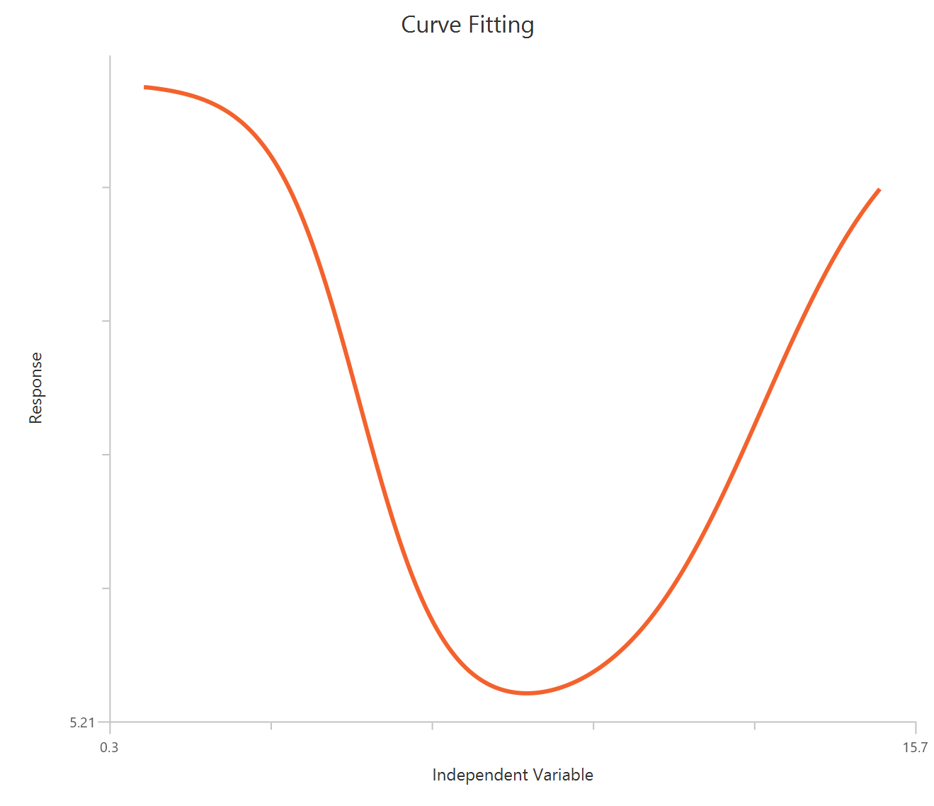
Biphasic, X is Concentration

TheBiphasic, X is Concentration is used when the response shows two distinct phases across the concentration range, consistent with two components of different potency and/or direction. The observed curve is typically modeled as the sum of two Hill-type terms, each with its own EC50 (and often its own amplitude), while sharing a common baseline. One phase may dominate at low concentrations and the other at higher concentrations, producing an inflection or “shoulder” that a single-site logistic cannot fit. This approach is often interpreted as reflecting two receptor populations, two binding sites, or mixed mechanisms, though the fit itself is phenomenological. Dense sampling across both transition regions is important to reliably resolve both components.

Equation

\[ \begin{equation} Span = Top - Bottom \end{equation} \]

\[ \begin{equation} \begin{alignedat}{2} Section_{1} = \frac{Span \cdot Frac}{(\frac{\mathrm{EC50}_{1}}{X})^{\mathrm{nH}_{1}} + 1} \qquad & Section_{2} = \frac{Span \cdot (-Frac + 1)}{(\frac{\mathrm{EC50}_{2}}{X})^{\mathrm{nH}_{2}} + 1} \end{alignedat} \end{equation} \]

\[ \begin{equation} Y = Bottom + Section_{1} + Section_{2} \end{equation} \]

Visualization

Input

The independent variable (X) must be the log10-transformed concentration/dose (i.e., \(𝑋 = log_{10}(concentration/dose)\)). The model also requires a column containing the dependent variable (Y) response values (in any consistent units).

Parameters

1. \(Bottom\): The lower asymptote (minimal response at very low concentration), typically reflecting baseline/background or fully inhibited activity.

2. \(Top\): The upper asymptote (maximal response at high concentration), i.e., the observed Emax or uninhibited plateau.

3. $\mathrm{EC50}_1$ and $\mathrm{EC50}_2$: represent the concentrations (expressed in the same units as X) at which each phase reaches 50% of its respective maximal effect — the first for the stimulatory component and the second for the inhibitory component.

4. \(nH_1\): The steepness factor for phase 1; captures apparent cooperativity/heterogeneity of the first component.

5. \(nH_2\): The steepness factor for phase 2; defines how sharply the second phase transitions.

---

Biphasic, X is log10(concentration)

The Biphasic, X is log10(concentration) is used when the response exhibits two separable phases across the concentration range that cannot be captured by a single sigmoidal curve. The observed profile is modeled as the sum of two Hill-type components sharing a common baseline, each with its own logEC50 (and typically its own amplitude and slope). Using a log-scaled X-axis expands the low-dose region, helping to resolve distinct transitions and “shoulders” between phases. This behavior is often consistent with two receptor populations, two binding sites, or mixed mechanisms, though the model remains phenomenological. Robust estimation requires data that cover both transition regions with sufficient points.

Equation

\begin{equation} Span = Top - Bottom \end{equation}

\[ \begin{equation} \begin{alignedat}{2} Section_{1} = \frac{Span \cdot Frac}{10^{\mathrm{nH}_{1} \cdot (\mathrm{LogEC50}_{1}-X)} + 1} \qquad & Section_{2} = \frac{Span \cdot (-Frac + 1)}{10^{\mathrm{nH}_{2} \cdot (\mathrm{LogEC50}_{2}-X)} + 1} \end{alignedat} \end{equation} \]

\begin{equation} Y = Bottom + Section_{1} + Section_{2} \end{equation}

Visualization

Input

The independent variable (X) must be the log10-transformed concentration/dose (i.e., \(𝑋 = log_{10}(concentration/dose)\)). The model also requires a column containing the dependent variable (Y) response values (in any consistent units).

Parameters

1. \(Bottom\): The lower asymptote (minimal response at very low concentration), typically reflecting baseline/background or fully inhibited activity.

2. \(Top\): The upper asymptote (maximal response at high concentration), i.e., the observed Emax or uninhibited plateau.

3. \(\mathrm{LogEC50}_{1}\) and \(\mathrm{LogEC50}_{2}\): denote the log-transformed concentrations (in the same units as X) at which each phase achieves 50% of its maximal effect — LogEC50_1 for the stimulatory component and LogEC50_2 for the inhibitory component.

4. \(nH_1\): The steepness factor for phase 1; captures apparent cooperativity/heterogeneity of the first component.

5. \(nH_2\): The steepness factor for phase 2; defines how sharply the second phase transitions.

---

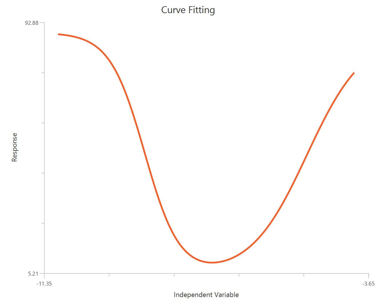
Bell-shaped, X is Concentration

The Bell-shaped dose-response model (X is concentration/dose) is used when a compound produces two opposing effects accross the concentration range, either stimulation at one range and inhibition at another or the reverse. The observed “bell” is modeled as the sum of two Hill-type dose-response curves that share a common baseline.

Equation

\[ \begin{equation} \begin{alignedat}{2} \mathrm{Span}_1 &= \mathrm{Plateau}_1 - \mathrm{Dip} \qquad & \mathrm{Span}_2 &= \mathrm{Plateau}_2 - \mathrm{Dip} \\ \mathrm{Section}_1 &= \frac{\mathrm{Span}_1}{1+(\mathrm{LogEC50}_1 - X)^{nH_1}} \qquad & \mathrm{Section}_2 &= \frac{\mathrm{Span}_2}{1+(X - \mathrm{LogEC50}_2)^{nH_2}} \\ \end{alignedat} \end{equation} \]

\begin{equation} Y = Dip + Section_1 + Section_2 \end{equation}

Visualization

Input

The independent variable (X) must be the concentration/dose on a linear scale and therefore must be strictly positive \((X>0)\). Zero or negative X values are not used in the calculations (they are ignored/excluded). The model also requires a column containing the dependent variable (Y) response values (in any consistent units).

Parameters

1. \(Dip\): The shared baseline (offset) of the whole model. The predicted response starts from Dip, and then the two components (Section1 and Section2) add to it.

2. \(Plateau_1\): Defines the asymptotic level used to set the amplitude of component 1. If \(Span_1 > 0\), component 1 contributes upward, otherwise downward.

3. \(EC50_1\)/\(IC50_1\): This is the concentration where component 1 is half-maximal. (\(nH_1\) > 0 → stimulation → parameter is \(EC50_1\), \(nH_1\) < 0 → inhibition → parameter is \(IC50_1\))

4. \(nH_1\): Controls the steepness of component 1 and the stimulation vs inhibition

5. \(Plateau_2\): Defines the asymptotic level used to set the amplitude of component 2. If \(Span_2 > 0\), component 2 contributes upward, otherwise downward.

6. \(EC50_2\)/\(IC50_2\): This is the concentration where component 2 is half-maximal. (\(nH_2\) > 0 → stimulation → parameter is \(EC50_2\), \(nH_2\) < 0 → inhibition → parameter is \(IC50_2\))

7. \(nH_2\): Controls the steepness of component 2 and the stimulation vs inhibition

---

Bell-shaped, X is log10(concentration)

The Bell-shaped dose-response model (X is log10 concentration/dose) is used when a compound produces two opposing effects accross the concentration range, either stimulation at one range and inhibition at another or the reverse. The observed “bell” is modeled as the sum of two Hill-type dose-response curves that share a common baseline.

Equation

\[ \begin{equation} \begin{alignedat}{2} \mathrm{Span}_1 &= \mathrm{Plateau}_1 - \mathrm{Dip} \qquad & \mathrm{Span}_2 &= \mathrm{Plateau}_2 - \mathrm{Dip} \\ \mathrm{Section}_1 &= \frac{\mathrm{Span}_1}{1+10^{(\mathrm{LogEC50}_1 - X)\,nH_1}} \qquad & \mathrm{Section}_2 &= \frac{\mathrm{Span}_2}{1+10^{(X-\mathrm{LogEC50}_2)\,nH_2}} \\ \end{alignedat} \end{equation} \]

\begin{equation} Y = Dip + Section_1 + Section_2 \end{equation}

Visualization

Input

The independent variable (X) must be the log10-transformed concentration/dose (i.e., \(𝑋 = log_{10}(concentration/dose)\)). The model also requires a column containing the dependent variable (Y) response values (in any consistent units).

Parameters

1. \(Dip\): The shared baseline (offset) of the whole model. The predicted response starts from Dip, and then the two components (Section1 and Section2) add to it.

2. \(Plateau_1\): Defines the asymptotic level used to set the amplitude of component 1. If \(Span_1 > 0\), component 1 contributes upward, otherwise downward.

3. \(LogEC50_1\)/\(LogIC50_1\): This is the log10 concentration where component 1 is half-maximal. (\(nH_1\) > 0 → stimulation → parameter is \(LogEC50_1\), \(nH_1\) < 0 → inhibition → parameter is \(LogIC50_1\))

4. \(nH_1\): Controls the steepness of component 1 and the stimulation vs inhibition

5. \(Plateau_2\): Defines the asymptotic level used to set the amplitude of component 2. If \(Span_2 > 0\), component 2 contributes upward, otherwise downward.

6. \(LogEC50_2\)/\(LogIC50_2\): This is the log10 concentration where component 2 is half-maximal. (\(nH_2\) > 0 → stimulation → parameter is \(LogEC50_2\), \(nH_2\) < 0 → inhibition → parameter is \(LogIC50_2\))

7. \(nH_2\): Controls the steepness of component 2 and the stimulation vs inhibition

---

Find ECF - Sigmoidal 4P, X is concentration

The Find ECF - Sigmoidal 4P, X is concentration analysis fits a standard sigmoidal concentration–response curve using linear agonist concentration on the X-axis, then reports the concentration producing a user-defined effect level (ECx). Instead of restricting output to EC50, it interpolates (or extrapolates, if allowed) the agonist concentration at x% of the response range between Bottom and Top (or another specified reference). The underlying fit typically estimates Top, Bottom, EC50, and a slope term (fixed or variable, depending on settings), and then computes ECanything from that fitted curve. Because X is linear, reliable ECx estimates require sufficient data density in the region surrounding the target response level. This method is useful for reporting regulatory or pharmacological endpoints such as EC10, EC20, EC80, etc., on a consistent model basis.

Equation

\begin{equation} \mathrm{EC50} = \frac{\mathrm{ECF}}{(\frac{F}{-F+100})^{\frac{1}{\mathrm{HillSlope}}}} \end{equation}

\begin{equation} Y = \mathrm{Bottom} + \frac{\mathrm{Top} - \mathrm{Bottom}}{(\frac{\mathrm{EC50}}{X})^{\mathrm{HillSlope}} + 1} \end{equation}

Visualization

Input

The independent variable (X) must be the agonist concentration on a linear scale (i.e., X=[agonist], in any consistent concentration units). The model also requires a column containing the dependent variable (Y) response values (in consistent response units, e.g., % effect or signal). This analysis additionally requires specification of one extra setting:

• \(ECx level (x%)\): The target effect level at which to report ECanything (e.g., EC10, EC20, EC80), defined as x% of the fitted response range between Bottom and Top (or relative to the chosen baseline/normalization convention).

Parameters

1. \(ECF\) (\(EC_{anything}\)): The agonist concentration that produces a response at F% of the span between Bottom and Top (e.g., F=80 gives EC80). The software typically reports both ECF and logECF.

2. \(HillSlope\): The slope (steepness) parameter of the sigmoidal curve; values >1 indicate a steeper transition and values <1 a shallower transition, with 1.0 often used as a standard constraint.

3. \(Top\) /\(Bottom\): The upper and lower plateaus of the response (in Y-units), defining the dynamic range used to compute the F% effect level.

4. \(F\): The user-specified target effect percentage that defines “ECanything” (e.g., 10, 20, 50, 80), interpreted relative to the fitted Bottom-to-Top range.

---

Find ECF - Sigmoidal 4P, X is log10(concentration)

The Find ECF - Sigmoidal 4P, X is log10(concentration) analysis fits a standard sigmoidal concentration–response curve with \(X = log_{10}(agonist)\) and then reports the agonist level that produces a user-defined effect (ECF/ECx). Rather than limiting the output to EC50, it computes the concentration giving F% of the fitted response range between Bottom and Top (e.g., EC10, EC80). The underlying fit estimates Bottom, Top, and HillSlope, and uses the fitted curve to interpolate the corresponding logECF (and ECF). Log-scaling expands the low-dose region, typically improving precision for EC values on the lower part of the curve. This approach is useful for standardized potency reporting at specific effect levels across conditions.

Equation

\begin{equation} \mathrm{LogEC50} = \mathrm{LogECF} - \frac{\mathrm{Log(\frac{F}{-F + 100})}}{\mathrm{HillSlope}} \end{equation}

\begin{equation} Y = \mathrm{Bottom} + \frac{\mathrm{Top} - \mathrm{Bottom}}{10^{\mathrm{HillSlope} \cdot (\mathrm{LogEC50} - X)} + 1} \end{equation}

Visualization

Input

The independent variable (X) must be the agonist concentration on a log10 scale (i.e., \(X=log⁡_{10}(\mathrm{agonist})\), in any consistent concentration units). The model also requires a column containing the dependent variable (Y) response values (in consistent response units, e.g., % effect or signal). This analysis additionally requires specification of one extra setting:

• \(ECx_{level} (x\%)\): The target effect level at which to report ECanything (e.g., EC10, EC20, EC80), defined as x% of the fitted response range between Bottom and Top (or relative to the chosen baseline/normalization convention).

Parameters

1. \(ECF (ECanything)\): The agonist concentration that produces a response at F% of the span between Bottom and Top (e.g., F=80 gives EC80). The software typically reports both ECF and logECF.

2. \(HillSlope\): The slope (steepness) parameter of the sigmoidal curve; values >1 indicate a steeper transition and values <1 a shallower transition, with 1.0 often used as a standard constraint.

3. \(Top\) /\(Bottom\): The upper and lower plateaus of the response (in Y-units), defining the dynamic range used to compute the F% effect level.

4. \(F\): The user-specified target effect percentage that defines “ECanything” (e.g., 10, 20, 50, 80), interpreted relative to the fitted Bottom-to-Top range.

---

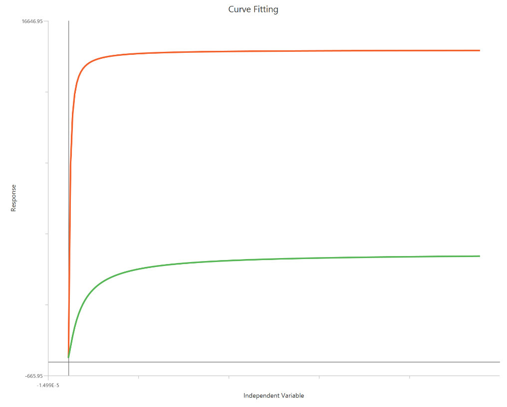
Operational model - Receptor depletion, X is Concentration

The Operational model — receptor depletion (X is concentration) is an extension of the Black–Leff operational model used to quantify agonism when the functional response is measured after reducing the available receptor population (e.g., irreversible antagonist or alkylation). By incorporating a depletion term (often expressed as the fraction of receptors remaining), the model separates affinity ($K_{a}$) from efficacy (τ, transducer ratio) and predicts how curves shift and depress as receptor reserve is removed. Fitting concentration–response data before/after depletion allows estimation of system-dependent amplification and agonist intrinsic efficacy, not just EC50 and Emax. It is especially useful for distinguishing partial agonism from limited receptor availability in the assay system.

Equation

\begin{equation} operate = {(\frac{\mathrm{K}_{a} + X}{\mathrm{T}_{au} \cdot X})}^n \end{equation}

\begin{equation} Y = \mathrm{Basal} + \frac{\mathrm{Effect}_{max} - \mathrm{Basal}}{\mathrm{operate} + 1} \end{equation}

Visualization

Input

The independent variable (X) must be on a linear scale and therefore must be strictly positive \((X>0)\). Zero or negative X values are not used in the calculations (they are ignored/excluded). This model requires two dependent-variable columns: one for no depletion and one depletion , both in consistent units. The two datasets must correspond to the same \(X\) values (or overlapping \(X\) ranges) so they can be fitted.

Parameters

1. \(Effect_{max}\): The system’s maximal achievable response (Y-units), i.e., the upper limit of the assay when receptors are not depleted and the agonist can drive the system to saturation.

2. \(Basal\): The response in the absence of agonist (baseline, Y-units); often fixed to 0 if data have been baseline-subtracted.

3. \(K_a\): The agonist–receptor dissociation constant (X-units), a direct index of affinity; it is mechanistically distinct from EC50, which is system-dependent.

4. \(T_{au}\): The transducer ratio/operational efficacy parameter describing coupling efficiency and receptor reserve; larger tau implies less occupancy is needed to generate a given effect.

5. \(n\): A unitless transducer slope (shape) parameter controlling the steepness of the operational stimulus–response relationship; it is related to, but not the same as, a Hill slope.

---

Operational model - Receptor depletion, X is log10(concentration)

The Operational model — receptor depletion (\(X = log_{10}(concentration)\)) applies the Black–Leff operational framework to concentration–response data collected before and after reducing the available receptor population. Using a log-scaled X-axis expands the low-dose region and facilitates comparison of curve shifts and Emax depression produced by depletion. The model estimates $K_{a}$ (agonist affinity) and τ (operational efficacy/transducer ratio), often alongside Basal, Effectmax, and an optional transducer slope (n). By explicitly accounting for receptor reserve, it can separate true affinity/efficacy from system amplification that confounds simple EC50/Emax fits.

Equation

\begin{equation} operate = {(\frac{10^{\mathrm{LogK}_{a}} + 10^{X}}{10^{\mathrm{LogT}_{au} + X}})}^n \end{equation}

\begin{equation} Y = \mathrm{Basal} + \frac{\mathrm{Effect}_{max} - \mathrm{Basal}}{\mathrm{operate} + 1} \end{equation}

Visualization

Input

The independent variable (X) can be entered on a log10 scale. In that case, X represents log10(concentration) values, which may be negative for concentrations below 1 in the chosen units, and these values are included in the fit. This model requires two dependent-variable columns: one for no depletion and one depletion, both in consistent units. The two datasets must correspond to the same \(X\) values (or overlapping \(X\) ranges) so they can be fitted.

Parameters

1. \(Basal\): The baseline response in the absence of agonist (constitutive/background signal), in Y-units.

2. \(Effect_{max}\): The maximal system response achievable in the assay (upper limit/Emax), in Y-units.

3. \(logK{a}\): The log10 of the agonist–receptor dissociation constant (affinity term); lower $K_{a}$ implies higher affinity.

4. \(LogT_{au}\): The log10 of the transducer ratio (tau), an operational measure of efficacy/coupling efficiency and receptor reserve; higher tau indicates greater efficacy.

5. \(n\): The unitless transducer slope (shape) parameter controlling the steepness of the stimulus–response mapping (related to, but distinct from, a Hill slope).

---

Operational model - Partial agonist, X is Concentration

The Operational model — Partial agonist (X is Concentration) applies the Black–Leff framework to agonists that produce a submaximal effect even at full receptor occupancy. Using linear concentration on the X-axis, the model relates stimulus to response through affinity (\({K}_{a}\)) and operational efficacy (τ) rather than relying solely on EC50/Emax. It predicts both rightward shifts and reduced Emax relative to a full agonist, allowing separation of binding affinity from functional efficacy. The formulation can include Basal, Effectmax, and an optional transducer slope (n) to describe curve shape. This model is particularly useful for comparing partial vs. full agonists within the same receptor system.

Equation

\begin{equation} operate = {(\frac{\mathrm{K}_{a} + X}{\mathrm{T}_{au} \cdot X})}^n \end{equation}

\begin{equation} \begin{alignedat}{2} \mathrm{Y}_{\mathrm{\langle A \rangle}} &= \mathrm{Basal} + \frac{\mathrm{Effect}_{max} - \mathrm{Basal}}{\left(\dfrac{\mathrm{EC}_{50}}{X}\right)^{n} + 1} \qquad & \mathrm{Y}_{\mathrm{\langle \sim A \rangle}} &= \mathrm{Basal} + \frac{\mathrm{Effect}_{max} - \mathrm{Basal}}{\mathrm{operate} + 1} \end{alignedat} \end{equation}

Visualization

Input

The independent variable (X) must be on a linear scale and therefore must be strictly positive \((X>0)\). Zero or negative X values are not used in the calculations (they are ignored/excluded). This model requires two dependent-variable columns: one for full and one partial agonist, both in consistent units. The two datasets must correspond to the same \(X\) values (or overlapping \(X\) ranges) so they can be fitted.

Parameters

1. \(Effect_{max}\): The maximum response the system can produce (Y-units), defined by the upper plateau of the full agonist concentration–response curve.

2. \(Basal\): The response measured with no agonist present (baseline, Y-units); if you baseline-corrected the data, it is often fixed to 0.

3. \(n\): A unitless transducer slope/shape parameter that governs curve steepness; it is related to, but not identical with, the Hill slope and is often constrained to 1.0.

4. \(\mathrm{K}_{a}\) (and \(\mathrm{LogK}_{a}\)): The equilibrium dissociation constant of the partial agonist (same units as X), quantifying binding affinity; Prism commonly reports both $K_{a}$ and its log10 value.

5. \(T_{au}\): The transducer ratio, an operational index of efficacy/coupling efficiency; it reflects how much receptor occupancy is required to generate a given response, and Prism may report both τ and log10(tau).

6. \(EC50\): The agonist concentration (in the same units as X) that produces 50% of the maximal response range between Basal (or Bottom) and Effectmax (or Top); a direct measure of potency.

---

Operational model - Partial agonist, X is log10(concentration)

The Operational model — receptor depletion (\(X = log_{10}(concentration)\)) applies the Black–Leff operational framework to datasets collected before and after reducing receptor availability (e.g., irreversible antagonist treatment). With a log-scaled X-axis, the low-dose region is expanded, improving definition of the transition and facilitating comparison of rightward shifts and Emax depression caused by depletion. The model estimates $logK_{a}$ (affinity) and logtau/tau (operational efficacy/transducer ratio), typically alongside Basal, Effectmax, and an optional transducer slope (n). By explicitly accounting for receptor reserve, it separates ligand properties from system amplification more effectively than standard EC50/Emax fits.

Equation

\begin{equation} operate = {(\frac{10^{\mathrm{logK}_{a}} + 10^{X}}{10^{\mathrm{logT}_{au} + X}})}^n \end{equation}

\begin{equation} \begin{alignedat}{2} \mathrm{Y}_{\mathrm{\langle A \rangle}} &= \mathrm{Basal} + \frac{\mathrm{Effect}_{max} - \mathrm{Basal}}{10^{n \cdot (\mathrm{LogEC}_{50} - X)} + 1} \qquad & \mathrm{Y}_{\mathrm{\langle \sim A \rangle}} = \mathrm{Basal} + \frac{\mathrm{Effect}_{max} - \mathrm{Basal}}{\mathrm{operate} + 1} \end{alignedat} \end{equation}

Visualization

Input

The independent variable (X) can be entered on a log10 scale. In that case, X represents log10(concentration) values, which may be negative for concentrations below 1 in the chosen units, and these values are included in the fit. This model requires two dependent-variable columns: one for full and one partial agonist, both in consistent units. The two datasets must correspond to the same \(X\) values (or overlapping \(X\) ranges) so they can be fitted.

Parameters

1. \(Basal\): The baseline response in the absence of agonist (background/constitutive signal), in Y-units.

2. \(Effect_{max}\): The maximal system response achievable (upper limit of the assay, Y-units), typically defined under no-depletion conditions.

3. \(LogK_{a}\): The log10 of the agonist–receptor dissociation constant (affinity); lower Kₐ (higher log affinity) indicates tighter binding.

4. \(LogT_{au}\): The log10 of the transducer ratio τ, an operational index of efficacy/coupling efficiency and receptor reserve; higher values imply greater efficacy.

5. \(n\): A unitless transducer slope parameter controlling the steepness of the operational stimulus–response relationship; often constrained to 1.0.

6. \(LogEC50\): The \(log10\) agonist concentration that produces 50% of the response range between Bottom and Top (or Basal and Effectmax, depending on the model); it is a standard index of potency.

---

Gaddum/Schild EC50 shift, X is concentration

The Gaddum/Schild EC50 shift model (X is concentration) fits a family of agonist concentration–response curves measured at fixed antagonist concentrations to quantify competitive antagonism. Under surmountable competition, the agonist curves show parallel rightward shifts (increased EC50) with minimal change in maximal response. The shift is summarized by the dose ratio (EC50′/EC50) at each antagonist level and related to antagonist concentration via the Gaddum/Schild relationship. From these shifts, the model estimates antagonist affinity as $K_{B}$ (often reported as $pA_2 = −log_{10}$ $K_{B}$ when consistent with Schild theory). Using linear X makes accurate sampling around each EC50 especially important for reliable dose-ratio estimates.

Equation

\begin{equation} Antag = {(\frac{B}{10^{-\mathrm{pA}_{2}}})}^{\mathrm{SchildSlope}} + 1 \end{equation}

\begin{equation} Y = \mathrm{Bottom} + \frac{\mathrm{Top} - \mathrm{Bottom}} {\left(\frac{\mathrm{EC50}\cdot \mathrm{Antag}}{X}\right)^{\mathrm{HillSlope}} + 1} \end{equation}

Visualization

Input

The independent variable (X) must be on a linear concentration scale and therefore strictly positive (\(X>0\)). Zero or negative X values are excluded from the calculations. The dependent variable (Y) should contain the agonist response (e.g., % effect or response units) measured across the agonist concentration range. This is a global fit across multiple agonist dose–response curves: one control curve (no antagonist) and additional curves collected at fixed antagonist concentrations ([B]). Provide one Y column for the control and one Y column for each antagonist level; the antagonist concentrations must be entered consistently (same units as $K_{B}$). The curves should share overlapping X ranges so the EC50 shifts (dose ratios) can be estimated reliably.

Parameters

1. \(EC50\) / \(LogEC50\): EC50 is the agonist concentration producing a half-maximal response in the absence of antagonist (potency). logEC50 is the log10 of that value (in the same “log units” used to label X), while EC50 is the antilog in concentration units.

2. \(pA_{2}\): The negative log10 of the antagonist concentration that causes a twofold rightward shift of the agonist EC50 (dose ratio = 2). If SchildSlope = 1, $pA_2$ corresponds to \(pK_B\) (\(−log10 K_B\)).

3. \(A_{2}\): The antagonist concentration that produces a twofold EC50 shift (dose ratio = 2). When \(SchildSlope = 1\), A2 equals $K_{B}$ (equilibrium dissociation constant of the antagonist).

4. \(HillSlope\): The slope factor controlling the steepness of the agonist concentration–response curve; commonly constrained to 1 for standard sigmoidal behavior.

5. \(SchildSlope\): Describes how closely the EC50 shifts follow the competitive antagonism prediction; values near 1 indicate simple competition, whereas deviations suggest non-ideal behavior.

6. \(Top\) /\(Bottom\): The upper and lower plateaus of the response, in Y-units, assumed to be shared across curves when shifts are purely horizontal.

---

Gaddum/Schild EC50 shift, X is log10(concentration)

The Gaddum/Schild EC50 shift model (\(X = log_{10}(concentration)\)) analyzes families of agonist concentration–response curves measured at fixed antagonist concentrations under a competitive antagonism framework. On a log-scaled X-axis, the curves are expected to show parallel rightward shifts with little or no change in Top/Bottom when antagonism is purely surmountable. The fit quantifies the shift via the dose ratio (EC50′/EC50) and estimates antagonist affinity as $pA_2$ (and, when SchildSlope ≈ 1, $pK_{B}$). Allowing SchildSlope to vary tests concordance with Schild theory, while HillSlope controls the steepness of the agonist response. This approach is widely used to infer $K_{B}$ from functional EC50 shifts rather than direct binding.

Equation

\begin{equation} \begin{alignedat}{2} Antag &= {(\frac{B}{10^{-\mathrm{pA}_{2}}})}^{\mathrm{SchildSlope}} + 1 \qquad & \mathrm{LogEC} &= \mathrm{Log(\mathrm{EC50} \cdot \mathrm{Antag})} \end{alignedat} \end{equation}

\begin{equation} Y = \mathrm{Bottom} + \frac{\mathrm{Top} - \mathrm{Bottom}}{10^{\mathrm{HillSlope} \cdot (\mathrm{LogEC} - X)} + 1} \end{equation}

Visualization

Input

The independent variable (X) is entered on a log10 concentration scale, so X represents log10[agonist] values. These values (which may be negative for concentrations below 1 in the chosen units) are included directly in the calculations. The dependent variable (Y) should contain the agonist response (e.g., % effect or response units) measured across the agonist concentration range. This is a global fit across multiple agonist dose–response curves: one control curve (no antagonist) and additional curves collected at fixed antagonist concentrations [B]. Provide one Y column for the control and one Y column for each antagonist level; the antagonist concentrations must be entered consistently (same units as $K_{B}$). The curves should share overlapping log X ranges so the EC50 shifts (dose ratios) can be estimated reliably.

Parameters

1. \(EC50\) / \(LogEC50\): EC50 is the agonist concentration producing a half-maximal response in the absence of antagonist (potency). logEC50 is the log10 of that value (in the same “log units” used to label X), while EC50 is the antilog in concentration units.

2. \(pA_{2}\): The negative log10 of the antagonist concentration that causes a twofold rightward shift of the agonist EC50 (dose ratio = 2). If SchildSlope = 1, $pA_2$ corresponds to \(pK_B\) (\(−log10 K_B\)).

3. \(A_{2}\): The antagonist concentration that produces a twofold EC50 shift (dose ratio = 2). When \(SchildSlope = 1\), A2 equals $K_{B}$ (equilibrium dissociation constant of the antagonist).

4. \(HillSlope\): The slope factor controlling the steepness of the agonist concentration–response curve; commonly constrained to 1 for standard sigmoidal behavior.

5. \(SchildSlope\): Describes how closely the EC50 shifts follow the competitive antagonism prediction; values near 1 indicate simple competition, whereas deviations suggest non-ideal behavior.

6. \(Top\) /\(Bottom\): The upper and lower plateaus of the response, in Y-units, assumed to be shared across curves when shifts are purely horizontal.

---

Gaddum/Schild EC50 shift (SchildSlope = 1), X is concentration

The Gaddum/Schild EC50 shift model with SchildSlope fixed to 1 (X is concentration) assumes simple, competitive, surmountable antagonism, so agonist curves exhibit parallel rightward shifts without changing Emax. With the Schild slope constrained, the relationship between antagonist concentration and dose ratio is fixed, and the fit focuses on estimating antagonist affinity as $K_{B}$ (often reported as $pK_{B}$/$pA_2$). The shift is quantified via the dose ratio (EC50′/EC50) computed from the fitted agonist curves at each antagonist level. Using linear X requires good sampling around each EC50 to estimate dose ratios accurately.

Equation

\begin{equation} Antag = \frac{B}{10^{-\mathrm{pA}_{2}}} + 1 \end{equation}

\begin{equation} Y = \mathrm{Bottom} + \frac{\mathrm{Top} - \mathrm{Bottom}} {\left(\frac{\mathrm{EC50}\cdot \mathrm{Antag}}{X}\right)^{\mathrm{HillSlope}} + 1} \end{equation}

Visualization

Input

The independent variable (X) must be on a linear concentration scale and therefore strictly positive \((X>0)\). Zero or negative X values are excluded from the calculations. The dependent variable (Y) should contain the agonist response (e.g., % effect or response units) measured across the agonist concentration range. This is a global fit across multiple agonist dose–response curves: one control curve (no antagonist) and additional curves collected at fixed antagonist concentrations ([B]). Provide one Y column for the control and one Y column for each antagonist level; the antagonist concentrations must be entered consistently (same units as $K_{B}$). The curves should share overlapping X ranges so the EC50 shifts (dose ratios) can be estimated reliably.

Parameters

1. \(EC50\) /\(LogEC50\): EC50 is the agonist concentration giving 50% of the maximal response in the absence of antagonist. logEC50 is the log10 form (in the same “log units” used for X labels), and EC50 is its antilog in concentration units.

2. \(pA_{2}\) ( \(= pK_B\) when \(SchildSlope = 1\)): The negative log10 of the antagonist concentration that produces a twofold rightward shift of the agonist curve; with SchildSlope fixed to 1 it directly reports antagonist affinity as \(pK_B\).

3. \(A_{2}\) ( \(= K_B\) when \(SchildSlope = 1\)): The antagonist concentration that yields a dose ratio of 2; when the Schild slope is constrained to 1, A2 is equivalent to\(K_B\) (equilibrium dissociation constant).

4. \(HillSlope\): Controls the steepness of the agonist concentration–response curves; it is often constrained to 1.0 to enforce standard sigmoidal behavior across the family of curves.

5. \(Top\) /\(Bottom\): The upper and lower response plateaus (in Y-units), defining the dynamic range and assumed to be common across curves when antagonism is purely surmountable.

---

Gaddum/Schild EC50 shift (SchildSlope = 1), X is log10(concentration)

The Gaddum/Schild EC50 shift model with SchildSlope fixed to 1 (\(X = log_{10}(concentration)\)) assumes simple competitive, surmountable antagonism, so agonist curves undergo parallel rightward shifts with no change in maximal response. With the Schild slope constrained, the fit directly links the dose ratio (EC50′/EC50) to antagonist concentration and estimates antagonist affinity as $K_{B}$ (often reported as $pK_{B}$, equivalent to $pA_2$ under this constraint). Using log10 X expands the low-dose region, improving definition of the transition around EC50 and the precision of the estimated shifts. This formulation is typically applied to a family of curves measured at fixed antagonist concentrations to obtain a single global affinity estimate.

Equation

\begin{equation} \begin{alignedat}{2} \mathrm{Antag} &= \frac{B}{10^{-\mathrm{pA}_{2}}} + 1 \qquad & \mathrm{LogEC50} &= Log(\mathrm{EC50}\cdot \mathrm{Antag}) \end{alignedat} \end{equation}

\begin{equation} Y = \mathrm{Bottom} + \frac{\mathrm{Top}-\mathrm{Bottom}}{10^{\mathrm{HillSlope} \cdot (\mathrm{LogEC} - X)} + 1} \end{equation}

Visualization

Input

The independent variable (X) is entered on a log10 concentration scale, so X represents log10[agonist] values. These values (which may be negative for concentrations below 1 in the chosen units) are included directly in the calculations. The dependent variable (Y) should contain the agonist response (e.g., % effect or response units) measured across the agonist concentration range. This is a global fit across multiple agonist dose–response curves: one control curve (no antagonist) and additional curves collected at fixed antagonist concentrations [B]. Provide one Y column for the control and one Y column for each antagonist level; the antagonist concentrations must be entered consistently (same units as $K_{B}$). The curves should share overlapping log X ranges so the EC50 shifts (dose ratios) can be estimated reliably.

Parameters

1. \(EC50\) /\(LogEC50\): EC50 is the agonist concentration giving 50% of the maximal response in the absence of antagonist. logEC50 is the log10 form (in the same “log units” used for X labels), and EC50 is its antilog in concentration units.

2. \(pA_2\) ( \(= pK_B\) when \(SchildSlope = 1\)): The negative log10 of the antagonist concentration that produces a twofold rightward shift of the agonist curve; with SchildSlope fixed to 1 it directly reports antagonist affinity as \(pK_B\).

3. \(A_2\) ( \(= K_B\) when \(SchildSlope = 1\)): The antagonist concentration that yields a dose ratio of 2; when the Schild slope is constrained to 1, A2 is equivalent to\(K_B\) (equilibrium dissociation constant).

4. \(HillSlope\): Controls the steepness of the agonist concentration–response curves; it is often constrained to 1.0 to enforce standard sigmoidal behavior across the family of curves.

5. \(Top\) /\(Bottom\): The upper and lower response plateaus (in Y-units), defining the dynamic range and assumed to be common across curves when antagonism is purely surmountable.

---

EC50 shift, X is concentration

The EC50 shift model (X is concentration) compares agonist concentration–response curves measured under control conditions and in the presence of a fixed modulator (e.g., antagonist) by quantifying the change in potency. The primary readout is the shift in EC50 (often expressed as an EC50 ratio or “dose ratio”), typically assuming the curves remain sigmoidal with similar HillSlope. In the simplest implementation, the modulator produces a horizontal displacement of the curve along the concentration axis, while Top and Bottom may be shared or allowed to vary depending on the mechanism. This approach is useful for summarizing potency changes without explicitly fitting a full Schild relationship. Reliable estimation requires dense sampling around each EC50 on the linear X-axis.

Equation

\begin{equation} \begin{alignedat}{2} \mathrm{EC}_{\langle A \rangle} &= \mathrm{EC50}_{Control} \qquad & \mathrm{EC}_{\langle \sim A \rangle} &= \mathrm{EC50}_{Control} \cdot \mathrm{EC50}_{Ratio} \end{alignedat} \end{equation}

\begin{equation} Y = \mathrm{Bottom} + \frac{\mathrm{Top} - \mathrm{Bottom}}{(\frac{EC}{X})^{\mathrm{HillSlope}} + 1} \end{equation}

Visualization

Input

The independent variable (X) must be on a linear scale and therefore must be strictly positive \((X>0)\). Zero or negative X values are not used in the calculations (they are ignored/excluded). This model requires two dependent-variable columns: one for no Inhibitor and one Inhibitor, both in consistent units. The two datasets must correspond to the same \(X\) values (or overlapping \(X\) ranges) so they can be fitted.

Parameters

1. \(EC50_{Control}\): The agonist concentration that produces a half-maximal response under control conditions (no modulator present), i.e., baseline potency.

2. \(Top / Bottom\): The upper and lower response plateaus (in Y-units), typically shared across curves to model a pure horizontal potency shift.

3. \(EC50_{Ratio}\): The fold-shift in potency, defined as \(EC50_{modulator} /EC50_{control}\); values >1 indicate a rightward shift (reduced potency).

4. \(HillSlope\): The shared slope parameter describing the steepness of the sigmoidal transition between Bottom and Top.

---

EC50 shift, X is log10(concentration)

The EC50 shift model (\(X = log_{10}(concentration)\)) analyzes a set of agonist concentration–response curves collected with and without a modulator by quantifying the change in potency on a log-scaled X-axis. The modulator effect is captured as an EC50 ratio (dose ratio), producing a horizontal displacement of the curve along log concentration. In the standard implementation, Top, Bottom, and HillSlope are shared across curves, so the fit isolates a pure EC50 shift without altering efficacy. Using log10 X expands the low-dose region and typically improves precision of the estimated shift around the midpoint. This approach provides a concise summary of modulator-induced potency changes without requiring a full Schild analysis.

Equation

\begin{equation} \begin{alignedat}{2} \mathrm{LogEC}_{\langle A \rangle} &= \mathrm{LogEC50}_{Control} \qquad & \mathrm{LogEC}_{\langle \sim A \rangle} &= \mathrm{LogEC50}_{Control} + \mathrm{LogEC50}_{Ratio} \end{alignedat} \end{equation}

\begin{equation} Y = \mathrm{Bottom} + \frac{\mathrm{Top} - \mathrm{Bottom}}{10^{\mathrm{HillSlope} \cdot (\mathrm{LogEC} - X)} + 1} \end{equation}

Visualization

Input

The independent variable (X) can be entered on a log10 scale. In that case, X represents log10(concentration) values, which may be negative for concentrations below 1 in the chosen units, and these values are included in the fit. This model requires two dependent-variable columns: one for no inhibitor and one inhibitor, both in consistent units. The two datasets must correspond to the same \(X\) values (or overlapping \(X\) ranges) so they can be fitted.

Parameters

1. \(EC50_{Control}\): The agonist concentration that produces a half-maximal response under control conditions (no modulator present), i.e., baseline potency.

2. \(Top / Bottom\): The upper and lower response plateaus (in Y-units), typically shared across curves to model a pure horizontal potency shift.

3. \(EC50_{Ratio}\): The fold-shift in potency, defined as \(EC50_{modulator} /EC50_{control}\); values >1 indicate a rightward shift (reduced potency).

4. \(HillSlope\): The shared slope parameter describing the steepness of the sigmoidal transition between Bottom and Top.

---

Allosteric EC50 shift, X is Concentration

The Allosteric EC50 shift model fits agonist dose–response curves measured at multiple fixed concentrations of an allosteric modulator (including a no-modulator control). The modulator does not directly generate a response; instead, it shifts the agonist’s apparent potency by changing the effective agonist concentration required to produce a given effect. The model globally estimates the agonist potency in the absence of modulator (EC50), the modulator affinity for its allosteric site (KB), and a cooperativity factor (\(a\)) that quantifies how modulator binding alters agonist potency. Curves shift left (\(a > 1\)) when the modulator increases agonist potency and shift right (\(α < 1\)) when it decreases potency.

Equation

\[ \begin{equation} \begin{alignedat}{2} \beta &= \frac{1+\mathrm{Allo}/K_B}{1+\alpha\,\mathrm{Allo}/K_B} \qquad & \mathrm{Antag} &= \mathrm{Agonist}\cdot \beta \\ Y &= \mathrm{Bottom} + \frac{\mathrm{Top}-\mathrm{Bottom}} {1+\left(\frac{\mathrm{EC50}}{\mathrm{Antag}}\right)^{\mathrm{HillSlope}}} \qquad & \end{alignedat} \end{equation} \]

(Here \(Allo\) is the fixed modulator concentration for each curve.)

Visualization

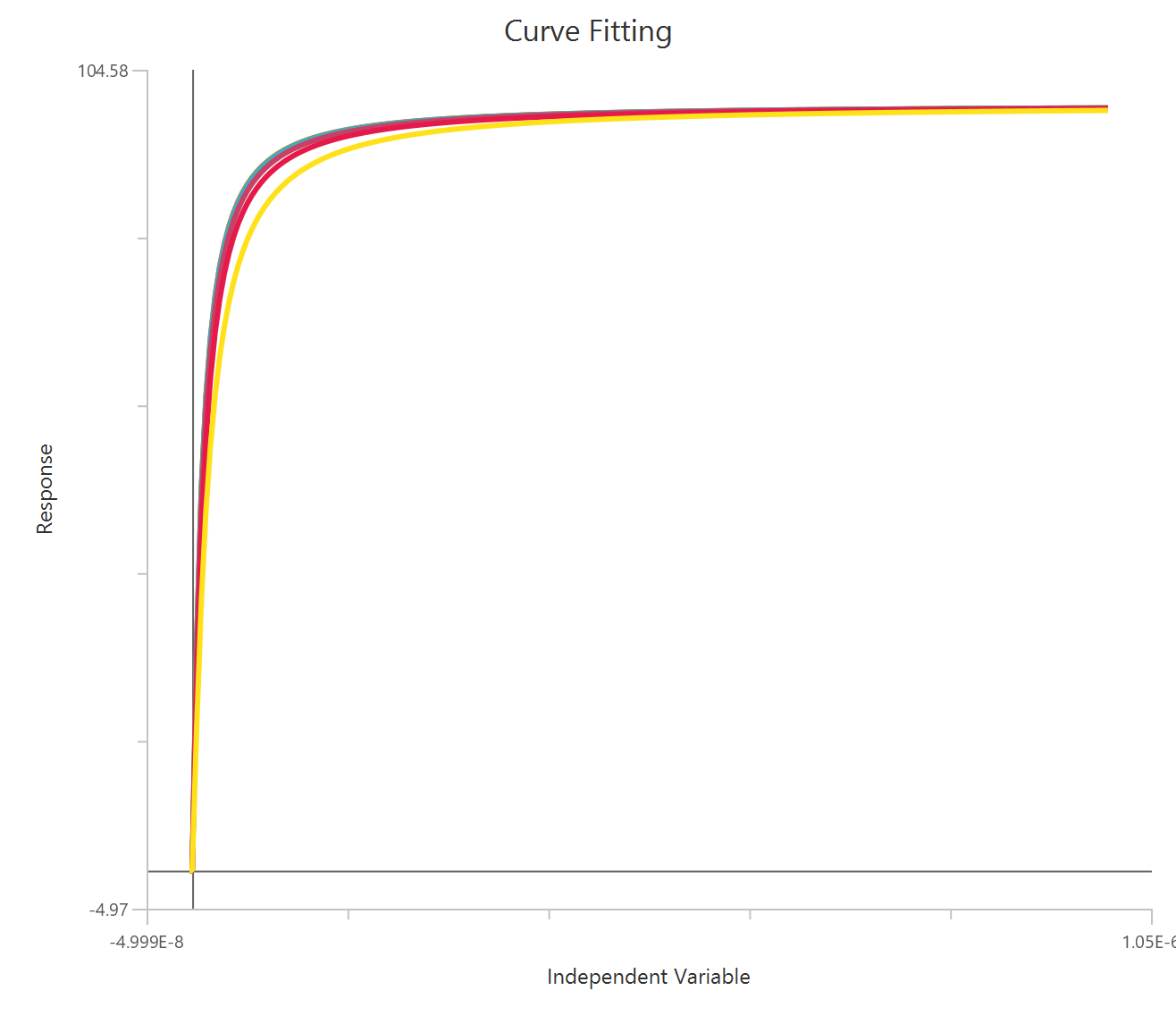
Input

The independent variable (X) must be the concentration/dose on a linear scale and therefore must be strictly positive \((X>0)\). Zero or negative X values are not used in the calculations (they are ignored/excluded). The dependent variable (Y) contains the measured response values. This is a global fit across multiple curves: each curve corresponds to a fixed modulator concentration (\(Allo\)). Provide one dataset with \(Allo=0\) (no modulator) and additional datasets for each modulator level, using consistent concentration units throughout.

Parameters

1. \(Top\): The upper plateau of the inhibition curve (response with no inhibitor / very low inhibitor). Same units as \(Y\).

2. \(Bottom\): The lower plateau approached by the tested inhibitor at high concentrations (residual response). Same units as \(Y\).

3. \(EC50\): Agonist concentration that produces half-maximal response in the absence of modulator. Same units as \(X\). Lower \(EC50\) indicates higher agonist potency.

4. \(HillSlope\): Controls the steepness of the curve transition.

5. \(KB\): Equilibrium dissociation constant (affinity) of the modulator for its allosteric site. Same molar units as \(Allo\). Lower \(KB\) indicates tighter modulator binding.

6. \(a\): Cooperativity factor describing how modulator binding changes agonist potency:

   1. \(a = 1\): no shift (modulator does not affect potency)
   2. \(a > 1\): left shift (agonist becomes more potent; EC50 decreases)
   3. \(a < 1\): right shift (agonist becomes less potent; EC50 increases)

---

Allosteric EC50 shift, X is log10(concentration)

The Allosteric EC50 shift model fits agonist dose–response curves measured at multiple fixed concentrations of an allosteric modulator (including a no-modulator control), when the agonist concentrations are entered as log₁₀ values. The modulator changes the apparent potency of the agonist without necessarily changing maximal efficacy, producing left- or right-shifts of the dose–response curves. By fitting all curves globally, the model estimates the agonist potency in the absence of modulator (logEC50), the modulator affinity for its site (logKB), and a cooperativity factor \((logAlpha / α)\) that quantifies how modulator binding alters agonist potency. Curves shift left when \(α>1\) and shift right when \(α<1\).

Equation

\[ \begin{equation} \begin{alignedat}{2} \mathrm{EC50} &= 10^{\mathrm{logEC50}} \qquad & K_B &= 10^{\mathrm{logKB}} \\ \alpha &= 10^{\mathrm{logAlpha}} \qquad & \mathrm{Antag} &= \frac{1+\mathrm{Allo}/K_B}{1+\alpha\,\mathrm{Allo}/K_B} \\ \mathrm{LogEC} &= \log_{10}\!\left(\frac{\mathrm{EC50}}{\mathrm{Antag}}\right) \qquad & \end{alignedat} \end{equation} \]

\[ \begin{equation} Y=\mathrm{Bottom}+\frac{\mathrm{Top}-\mathrm{Bottom}}{1+10^{(\mathrm{LogEC}-X)\cdot \mathrm{HillSlope}}} \end{equation} \]

(Here \(Allo\) is the fixed modulator concentration for each curve.)

Visualization

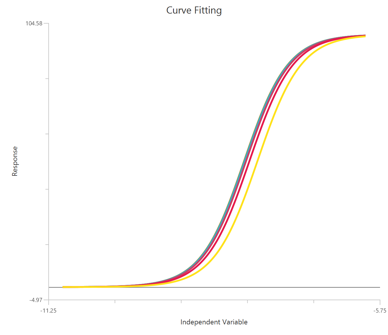
Input

The independent variable (X) must be the log₁₀-transformed agonist concentration (\(X = log_{10}(agonist)\)).. The dependent variable (Y) contains the measured response values. This is a global fit across multiple curves: each curve corresponds to a fixed modulator concentration (\(Allo\)). Provide one dataset with \(Allo=0\) (no modulator) and additional datasets for each modulator level, using consistent concentration units throughout.

Parameters

1. \(Top\): The upper plateau of the inhibition curve (response with no inhibitor / very low inhibitor). Same units as \(Y\).

2. \(Bottom\): The lower plateau approached by the tested inhibitor at high concentrations (residual response). Same units as \(Y\).

3. \(logEC50\): The base-10 logarithm of the agonist concentration that produces half-maximal response in the absence of modulator.

4. \(HillSlope\): Controls the steepness of the curve transition.

5. \(logKB\): The base-10 logarithm of the equilibrium dissociation constant for the modulator binding to its allosteric site.

6. \(logAlpha\): The base-10 logarithm of the cooperativity factor a:

   1. \(a = 1\): no shift (modulator does not affect potency)
   2. \(a > 1\): left shift (agonist becomes more potent; EC50 decreases)
   3. \(a < 1\): right shift (agonist becomes less potent; EC50 increases)

---

Absolute IC/EC50, X is Concentration

The Absolute IC/EC50 (X is concentration) model fits an inhibitory/stimulatory dose–response curve when you want the IC50/EC50 defined relative to a fixed reference baseline rather than relative to the fitted Bottom plateau. In many assays, the “fully inhibited” level is determined by a standard inhibitor / positive control (or another external reference) and may not coincide with the Bottom plateau reached by the tested compound. This model therefore distinguishes between Bottom (the asymptote of the tested compound) and Baseline (the externally defined 100% inhibition reference). The fitted Absolute IC50 is the concentration at which the response falls halfway between Top (no inhibitor) and Baseline (maximal inhibition reference), while the rest of the curve (Top, Bottom, HillSlope) is fitted to the data.

Equation

\[ \begin{equation} \begin{alignedat}{2} \mathrm{Fifty} &= \frac{\mathrm{Top}+\mathrm{Baseline}}{2} \qquad & \\ \mathrm{Scale} &= \frac{\mathrm{Top}-\mathrm{Bottom}}{\mathrm{Fifty}-\mathrm{Bottom}}-1 \qquad & \end{alignedat} \end{equation} \]

\[ \begin{equation} Y=\mathrm{Bottom}+\frac{\mathrm{Top}-\mathrm{Bottom}}{1+\left(\mathrm{Scale}\cdot\left(\frac{\mathrm{AbsoluteIC50}}{X}\right)\right)^{\mathrm{HillSlope}}} \end{equation} \]

Visualization

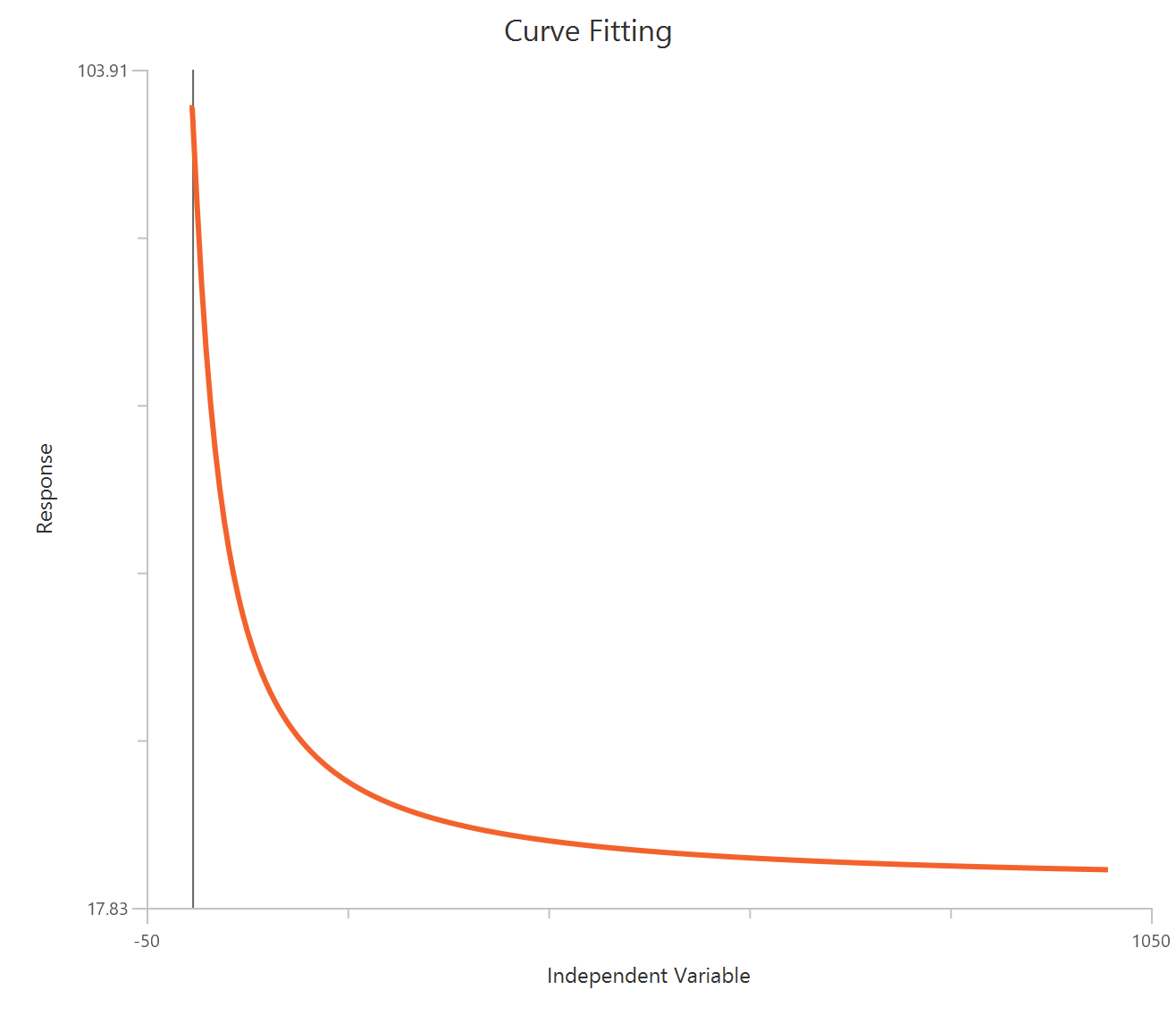
Input

The independent variable (X) must be the concentration/dose on a linear scale and therefore must be strictly positive \((X>0)\). Zero or negative X values are not used in the calculations (they are ignored/excluded). The model also requires a column containing the dependent variable (Y) response values (in any consistent units). This equation also requires the specification of one extra parameter:

1. \(Baseline\): The response level corresponding to maximal inhibition defined by a standard control (e.g., a reference inhibitor). It is used to define “100% inhibition” for the purpose of computing Absolute IC50. Baseline must be provided by the user and is in the same units as \(Y\).

Parameters

1. \(Top\): The upper plateau of the inhibition curve (response with no inhibitor / very low inhibitor). Same units as \(Y\).

2. \(Bottom\): The lower plateau approached by the tested inhibitor at high concentrations (residual response). Same units as \(Y\).

3. \(AbsoluteIC50/AbsoluteEC50\): The inhibitor/stimulation concentration that produces a response halfway between Top and Baseline.

4. \(HillSlope\): Controls the steepness of the curve transition.

---

Absolute IC/EC50, X is log10(concentration)

The Absolute IC/EC50 (X is concentration) model fits an inhibitory/stimulatory dose–response curve when you want the IC50/EC50 defined relative to a fixed reference baseline rather than relative to the fitted Bottom plateau. In many assays, the “fully inhibited” level is determined by a standard inhibitor / positive control (or another external reference) and may not coincide with the Bottom plateau reached by the tested compound. This model therefore distinguishes between Bottom (the asymptote of the tested compound) and Baseline (the externally defined 100% inhibition reference). The fitted Absolute IC50 is the concentration at which the response falls halfway between Top (no inhibitor) and Baseline (maximal inhibition reference), while the rest of the curve (Top, Bottom, HillSlope) is fitted to the data. Here, \(X\) is \(log_{10}(concentration)\).

Equation

\[ \begin{equation} \begin{alignedat}{2} \mathrm{Fifty} &= \frac{\mathrm{Top}+\mathrm{Baseline}}{2} \qquad & \\ \mathrm{Shift} &= \log_{10}\!\left(\frac{\mathrm{Top}-\mathrm{Bottom}}{\mathrm{Fifty}-\mathrm{Bottom}}-1\right) \qquad & \end{alignedat} \end{equation} \]

\[ \begin{equation} Y = \mathrm{Bottom} + \frac{\mathrm{Top}-\mathrm{Bottom}} {1+10^{\big((\mathrm{LogAbsoluteIC50}-X)\cdot \mathrm{HillSlope} + \mathrm{Shift}\big)}} \end{equation} \]

Visualization

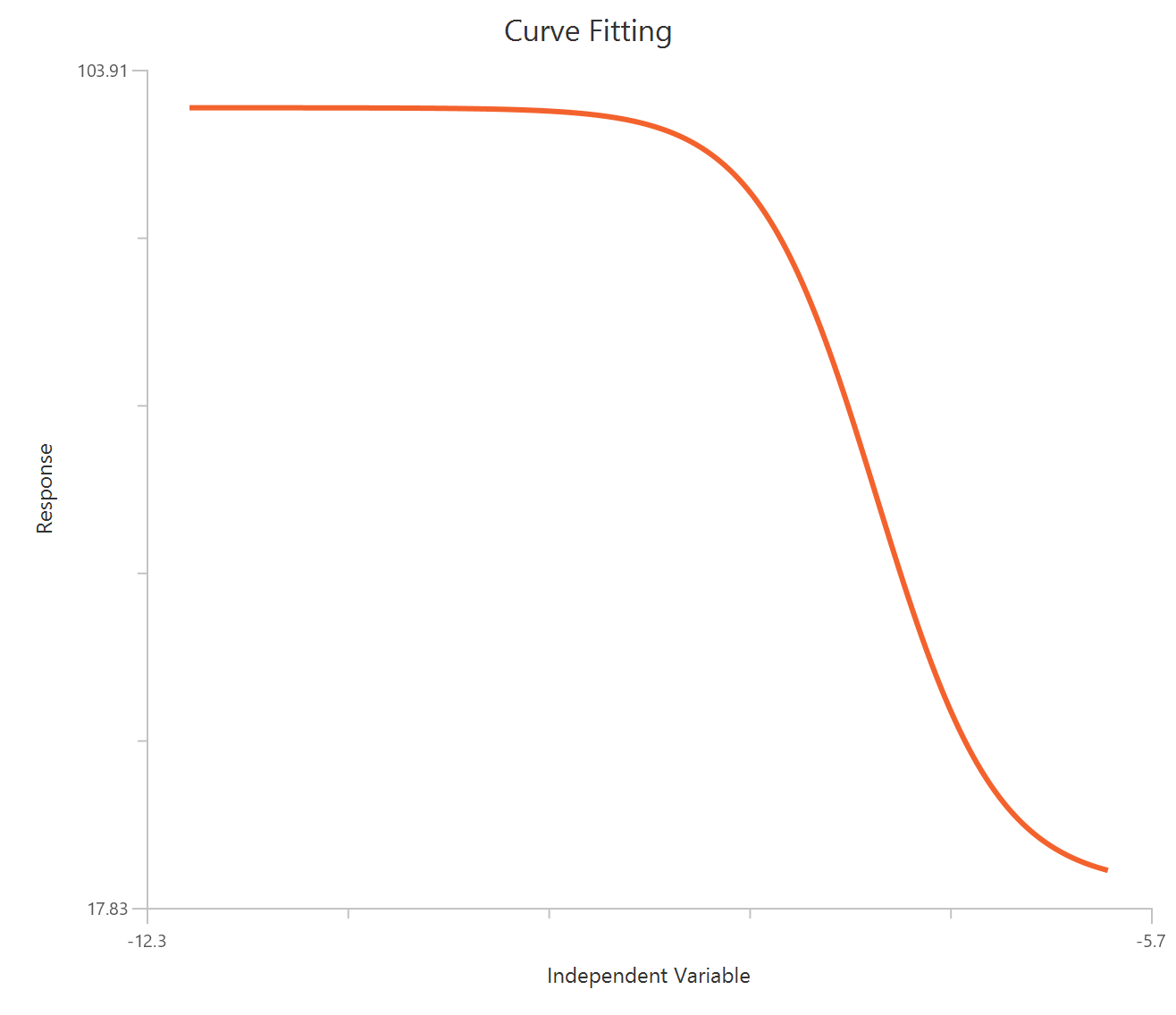
Input

The independent variable (X) must be the log10-transformed concentration/dose (i.e., \(𝑋 = log_{10}(concentration/dose)\)). The model also requires a column containing the dependent variable (Y) response values (in any consistent units). This equation also requires the specification of one extra parameter:

1. \(Baseline\): The response level corresponding to maximal inhibition defined by a standard control (e.g., a reference inhibitor). It is used to define “100% inhibition” for the purpose of computing Absolute IC50. Baseline must be provided by the user and is in the same units as \(Y\).

Parameters

1. \(Top\): The upper plateau of the inhibition curve (response with no inhibitor / very low inhibitor). Same units as \(Y\).

2. \(Bottom\): The lower plateau approached by the tested inhibitor at high concentrations (residual response). Same units as \(Y\).

3. \(LogAbsoluteIC50/LogAbsoluteEC50\): The \(log_{10}(concentration)\) that produces a response halfway between Top and Baseline.

4. \(HillSlope\): Controls the steepness of the curve transition.

---

Receptor Binding

One Site – Total

The One-site — Total binding model describes radioligand binding when the measured signal includes both specific binding to a single class of sites and nonspecific binding. Specific binding follows a one-site saturation isotherm and approaches a maximum capacity (Bmax) with increasing ligand concentration, with Kd equal to the ligand concentration that produces half-maximal specific binding. Nonspecific binding is assumed to increase linearly with ligand concentration, with slope NS, and an optional constant Background term accounts for baseline signal in the absence of added radioligand.

Equation

\begin{equation} Y = Bmax \frac{X}{K_d+X} + NS*X + Background \end{equation}

Visualization

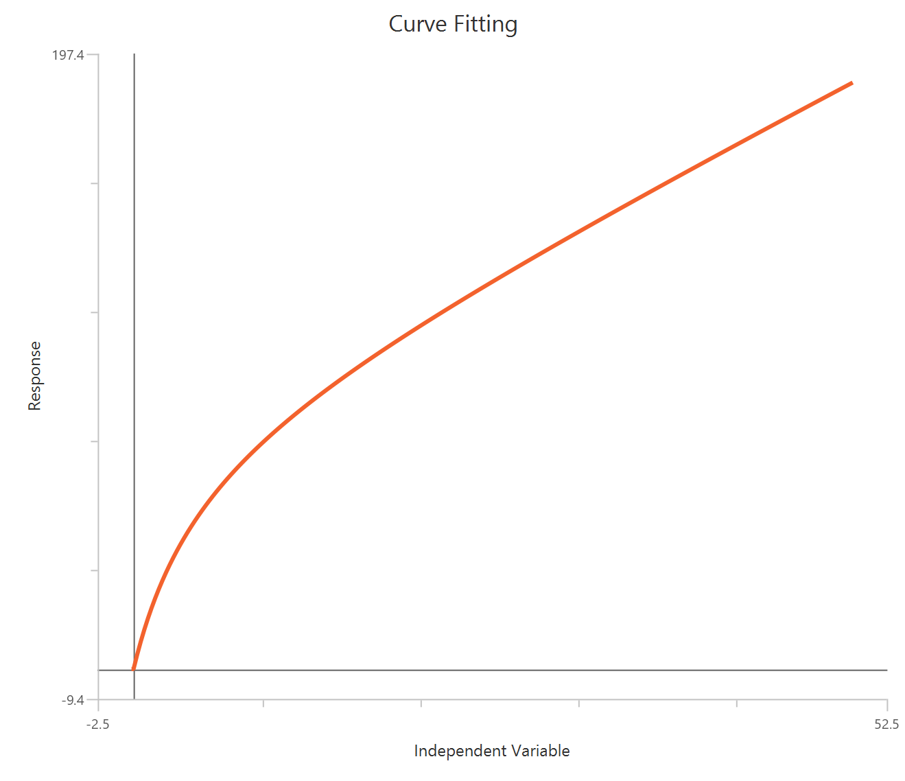
Input

The independent variable (X) must be on a linear scale and therefore must be strictly positive \((X>0)\). Zero or negative X values are not used in the calculations (they are ignored/excluded). The model also requires a column containing the dependent variable (Y) response values (in any consistent units).

Parameters

1. \(Bmax\): The shared baseline (offset) of the whole model. The predicted response starts from Dip, and then the two components (Section1 and Section2) add to it.

2. \(K_d\): The equilibrium dissociation constant of the ligand–site interaction. It is the concentration at which the specific binding term reaches 50% of Bmax; lower \(K_d\) indicates higher affinity.

3. \(NS\): The slope of nonspecific binding, assuming nonspecific binding increases linearly with concentration

4. \(Background\): A constant baseline offset in the measured signal (binding at \(X=0\)), representing instrument/counter background or residual signal not explained by specific or nonspecific binding.

---

One Site – Total, accounting for ligand depletion

The One site — Total, accounting for ligand depletion model fits total radioligand binding when a non-negligible fraction of ligand becomes bound, so the free ligand concentration is lower than the amount added (i.e., ligand depletion). Unlike the simple one-site total binding model (which assumes free ≈ added), this formulation explicitly accounts for depletion by solving the binding relationship using a quadratic expression.

Equation

\begin{equation} \mathrm{K_dCPM} = \mathrm{K_dNm}\cdot \mathrm{Vol}\cdot 1000 \cdot \mathrm{SpecAct} \qquad \end{equation}

\begin{equation} b = \mathrm{K_dCPM} + \mathrm{NS}\cdot \mathrm{K_dCPM} + X + 2X\cdot \mathrm{NS} + \mathrm{Bmax} \end{equation}

\begin{equation} c = -1\cdot X\left(\mathrm{NS}\cdot \mathrm{K_dCPM} + X\cdot \mathrm{NS} + \mathrm{Bmax}\right) \qquad \end{equation}

\[ \begin{equation} Y=\frac{-b+\sqrt{b^{2}-4ac}}{2a} \end{equation} \]

Visualization

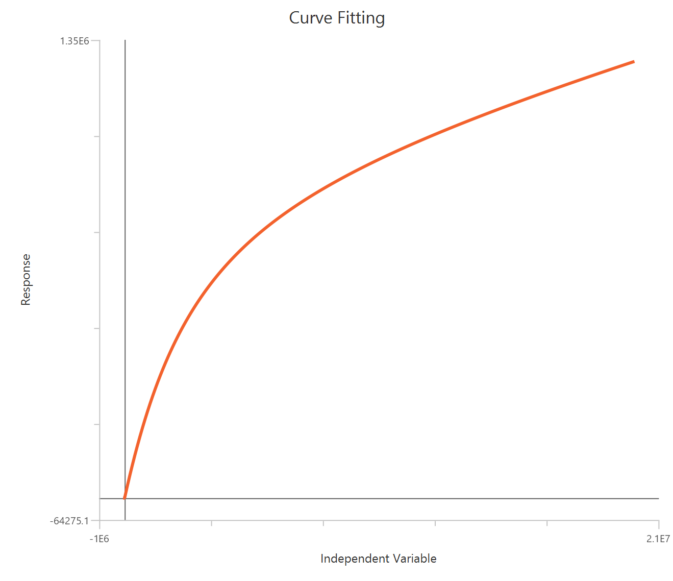
Input

The independent variable (X) must be on a linear scale and therefore must be strictly positive \((X>0)\). Zero or negative X values are not used in the calculations (they are ignored/excluded). The model also requires a column containing the dependent variable (Y) response values (in any consistent units). This equation also requires the specification of two extra parameters:

1. \(SpecAct\): The specific radioactivity (e.g., CPM per fmol). Used to convert concentrations into CPM units for the depletion calculation.
2. \(Vol\): The reaction volume (e.g., mL). Also used in the concentration → CPM conversion for KdCPM.

Parameters

1. \(Bmax\): The maximum specific binding capacity for the saturable one-site component. In this model it is reported in CPM (same units as \(Y\)).

2. \(K_dNm\): The equilibrium dissociation constant (affinity) in nM. It is the free-ligand concentration that produces half-maximal specific binding at equilibrium (lower \(K_d\) ⇒ higher affinity). Internally it is converted to \(K_dCPM\) using \(Vol\) and \(SpecAct\).

3. \(NS\): TThe slope of nonspecific binding, assuming nonspecific binding increases linearly with ligand. Units are effectively CPM per CPM in this formulation because both \(X\) and \(Y\) are in CPM (practically: “how much nonspecific signal rises as added ligand increases”).

---

One Site – Total and NonSpecific Binding

The One site — total and nonspecific binding model is used when you have measured total binding and nonspecific binding as separate data sets (typically under the same radioligand concentrations). The model fits both curves simultaneously: specific binding is described by a one-site saturation isotherm (\(Bmax,K_d\)), while nonspecific binding is modeled as a linear function of radioligand concentration. Total binding is then modeled as the sum of specific and nonspecific binding. Fitting the two data sets together improves identifiability because the nonspecific component is estimated directly from the nonspecific dataset while still contributing to the total binding fit.

Equation

\[ \begin{equation} \mathrm{Specific}(X) = \frac{\mathrm{Bmax}\,X}{\mathrm{Kd}+X} \end{equation} \] \[ \begin{equation} \mathrm{Nonspecific}(X) = \mathrm{NS}\cdot X + \mathrm{Background} \end{equation} \] \[ \begin{equation} \mathrm{Total}(X) = \mathrm{Specific}(X) + \mathrm{Nonspecific}(X) \end{equation} \]

\[ \begin{equation} \begin{aligned} Y_A = \mathrm{Total}(X) \quad Y_B = \mathrm{Nonspecific}(X) \end{aligned} \end{equation} \]

(Here \(Y_A\) corresponds to the total-binding dataset and \(Y_B\) corresponds to the nonspecific-binding dataset.)

Visualization

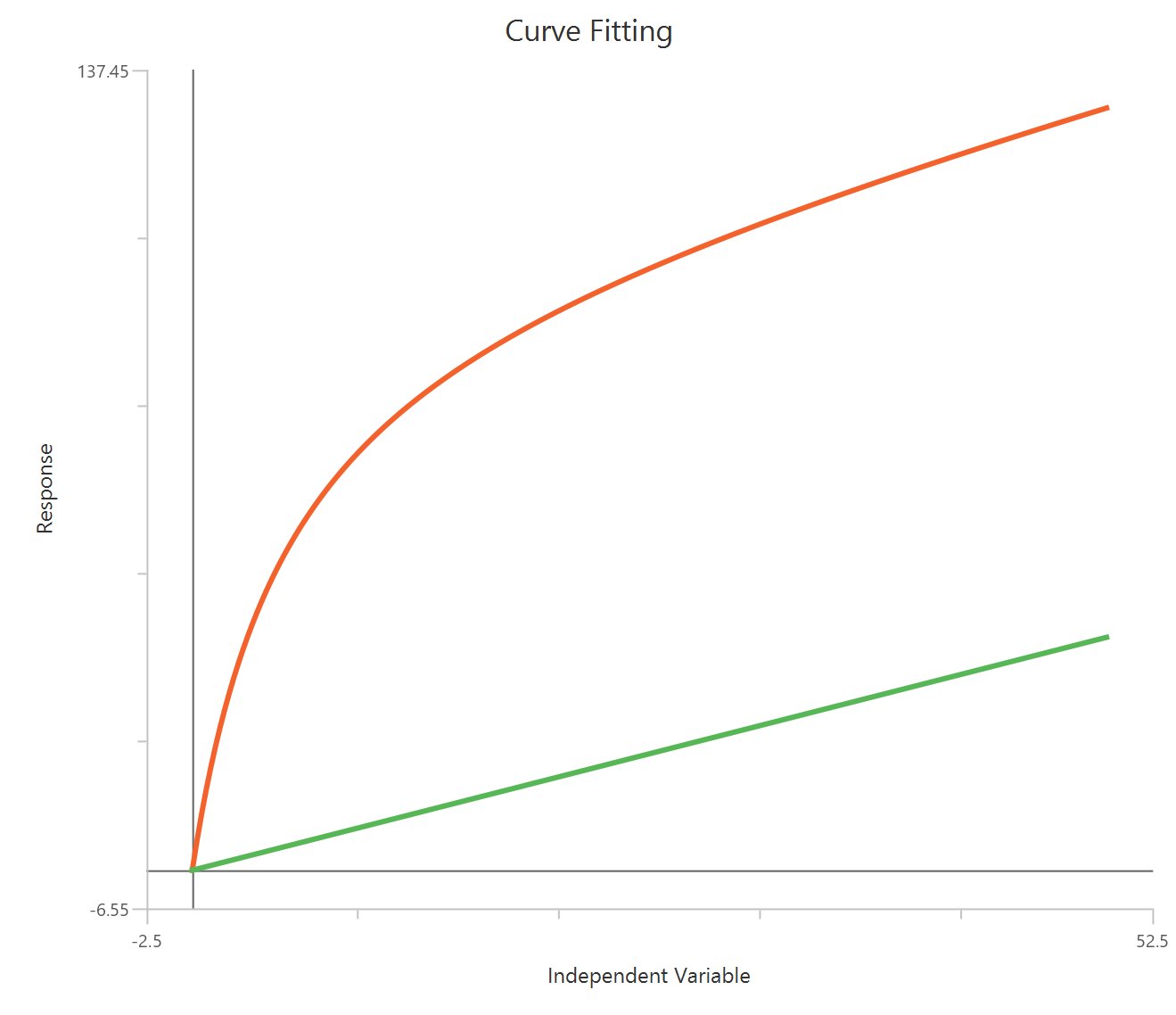
Input

The independent variable (X) must be on a linear scale and therefore must be strictly positive \((X>0)\). Zero or negative X values are not used in the calculations (they are ignored/excluded). This model requires two dependent-variable columns: one for total binding and one for nonspecific binding, both in consistent units. The two datasets must correspond to the same \(X\) values (or overlapping \(X\) ranges) so they can be fitted.

Parameters

1. \(Bmax\): The maximum specific binding capacity (the plateau of the saturable one-site component). Reported in the same units as the binding response \(Y\).

2. \(K_d\): The equilibrium dissociation constant (affinity), in the same units as \(X\). It is the radioligand concentration that produces half-maximal specific binding. Lower \(K_d\) indicates higher affinity.

3. \(NS\): TThe slope of nonspecific binding, assuming nonspecific binding increases linearly with ligand.

4. \(Background\): A constant baseline offset for nonspecific binding (binding when \(X=0\)). Often represents counter/instrument background or residual signal.

---

One Site – Specific Binding

The One site — Specific binding model describes binding to a single class of saturable sites after nonspecific binding has been removed from the data. Because only specific binding is analyzed, the response follows a simple one-site saturation isotherm that approaches a maximum (Bmax) as ligand concentration increases. The shape of the curve reflects reversible equilibrium binding, where binding rises steeply at low ligand concentrations and plateaus as receptors become saturated.

This model assumes that any nonspecific binding has already been subtracted (for example using a Remove Baseline analysis or by experimentally measuring and correcting for nonspecific binding). Consequently, the fitted curve represents only the receptor–ligand interaction, without a linear nonspecific component or background term.

Equation

\begin{equation} Y = \frac{BmaxX}{K_d+X} \end{equation}

Visualization

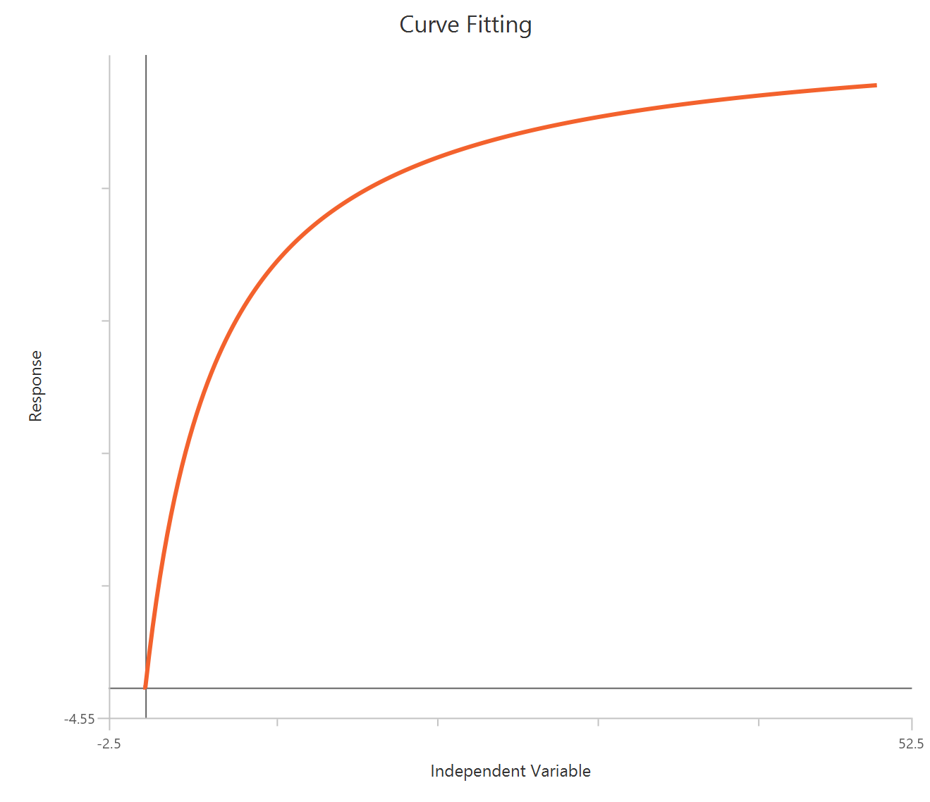
Input

The independent variable (X) must be on a linear scale and therefore must be strictly positive \((X>0)\). Zero or negative X values are not used in the calculations (they are ignored/excluded). The model also requires a column containing the dependent variable (Y) response values (in any consistent units).

Parameters

1. \(Bmax\): The shared baseline (offset) of the whole model. The predicted response starts from Dip, and then the two components (Section1 and Section2) add to it.

2. \(K_d\): The equilibrium dissociation constant of the ligand–site interaction. It is the concentration at which the specific binding term reaches 50% of Bmax; lower \(K_d\) indicates higher affinity.

---

Two Sites – Specific Binding

The Two sites — Specific binding model is used when the measured signal represents specific binding (i.e., nonspecific binding has already been removed) but the binding behavior cannot be explained by a single class of receptors. The model assumes there are two independent binding site populations (often interpreted as a high-affinity and a low-affinity site), each following a one-site saturation isotherm with its own capacity and affinity. The total specific binding is modeled as the sum of the two saturable components, producing a curve that can show an initially steep rise (high-affinity sites) followed by a broader approach to saturation (low-affinity sites).

Equation

\[ \begin{equation} \begin{alignedat}{2} \mathrm{Site}_\mathrm{Hi}(X) &= \frac{\mathrm{BmaxHi}\,*X}{\mathrm{KdHi}+X} \qquad & \mathrm{Site}_\mathrm{Lo}(X) &= \frac{\mathrm{BmaxLo}\,*X}{\mathrm{KdLo}+X} \\ \end{alignedat} \end{equation} \]

\[ \begin{equation} Y = \mathrm{Site}_\mathrm{Hi}(X) + \mathrm{Site}_\mathrm{Lo}(X) \end{equation} \]

Visualization

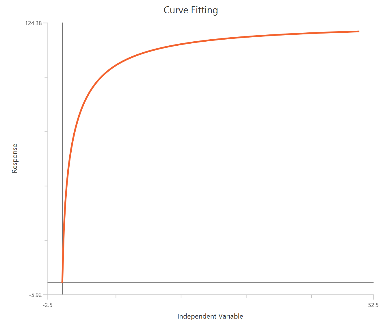
Input

The independent variable (X) must be on a linear scale and therefore must be strictly positive \((X>0)\). Zero or negative X values are not used in the calculations (they are ignored/excluded). The model also requires a column containing the dependent variable (Y) response values (in any consistent units).

Parameters

1. \(BmaxHi\): The maximum specific binding capacity of the high-affinity site population (plateau contribution from that site). Reported in the same units as \(Y\).

2. \(K_d^{Hi}\): The equilibrium dissociation constant for the high-affinity site population, in the same units as \(X\). It is the concentration that produces half-maximal binding for the high-affinity component . Lower \(K_d\) indicates higher affinity.

3. \(BmaxLo\): The maximum specific binding capacity of the low-affinity site population (plateau contribution from that site). Reported in the same units as \(Y\).

4. \(K_d^{Lo}\): The equilibrium dissociation constant for the low-affinity site population, in the same units as \(X\). It is the concentration that produces half-maximal binding for the low-affinity component . Lower \(K_d\) indicates higher affinity.

---

Allosteric Modulator Shift

The Allosteric Modulator Shift model describes radioligand binding to a single class of sites when an allosteric modulator is present at one or more fixed concentrations. Entire saturation binding curves are measured at each modulator level (including a no-modulator control). The model assumes the modulator binds to a distinct allosteric site and changes the apparent affinity of the radioligand via a cooperativity factor, \(α\). By fitting all curves globally, the model estimates the radioligand affinity in the absence of modulator, the modulator’s affinity for its site, and how strongly modulator binding shifts radioligand binding.

Equation

\[ \begin{equation} \begin{alignedat}{2} \mathrm{Hot} &= X \qquad & \alpha &= 10^{\mathrm{Log}\alpha} \\ K_B &= 10^{\mathrm{Log}K_B} \qquad & K_{\mathrm{App}} &= K_{d,\mathrm{Hot}}\, \frac{1+\mathrm{Allo}/K_B}{1+\alpha\,\mathrm{Allo}/K_B} \end{alignedat} \end{equation} \]

\[ \begin{equation} Y=\frac{\mathrm{Bmax}\cdot \mathrm{Hot}}{\mathrm{Hot}+K_{\mathrm{App}}} \end{equation} \]

(Here, \(Allo\) is the fixed modulator concentration for a given curve/column.)

Visualization

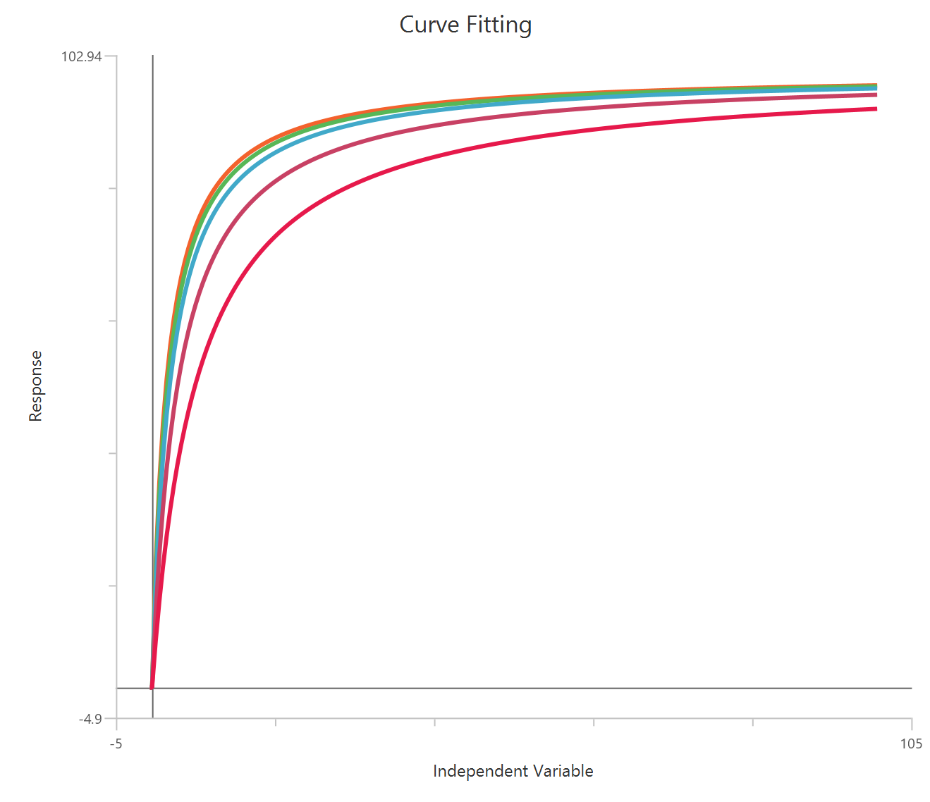
Input

The independent variable (X) must be on a linear scale and therefore must be strictly positive \((X>0)\). Zero or negative X values are not used in the calculations (they are ignored/excluded). The dependent variables (Y) should contain specific binding values. This is a global fit across multiple curves: each curve corresponds to a fixed allosteric modulator concentration (\(Allo\)). Provide one column for the no-modulator control and additional columns for binding measured at each modulator level. The modulator concentrations must be specified consistently (same units as \(KB\));

Parameters

1. \(Bmax\): The maximum specific binding capacity (plateau) of the radioligand saturation curve. Reported in the same units as \(Y\).

2. \(K_{d,Hot}\): The equilibrium dissociation constant of the radioligand in the absence of modulator, in the same units as \(X\). It is the radioligand concentration that gives half-maximal binding when \(Allo=0\).

3. \(K_B\): The equilibrium dissociation constant of the allosteric modulator for its allosteric site (affinity of the modulator). It is in the same molar units used for \(Allo\). Smaller \(K_B\) indicates tighter modulator binding.

4. \(alpha\): The cooperativity (ternary complex) factor that quantifies how modulator binding changes radioligand affinity.

   1. \(αlpha=1\): no shift (modulator does not change radioligand affinity)
   2. \(αlpha < 1\): apparent affinity of radioligand decreases (curve shifts right; less binding at a given \(X\)).
   3. \(alpha > 1\): apparent affinity of radioligand increases (curve shifts left; more binding at a given \(X\)).

---

Specific Binding with Hill Slope

The Specific binding with Hill slope model extends the one-site specific binding isotherm by allowing the curve’s steepness to vary through a Hill coefficient. It is used when nonspecific binding has already been removed and you are fitting specific binding only, but the transition from low to high binding is steeper or shallower than expected for simple 1:1 mass-action binding. The Hill slope (\(h\)) provides an empirical way to capture apparent cooperativity or heterogeneity in binding behavior, while still estimating the binding capacity (Bmax) and the concentration scale parameter (Kd).

Equation

\[ \begin{equation} \begin{alignedat}{2} Y &= \frac{\mathrm{Bmax}\,X^{h}}{\mathrm{Kd}^{h}+X^{h}} \qquad & \end{alignedat} \end{equation} \]

Visualization

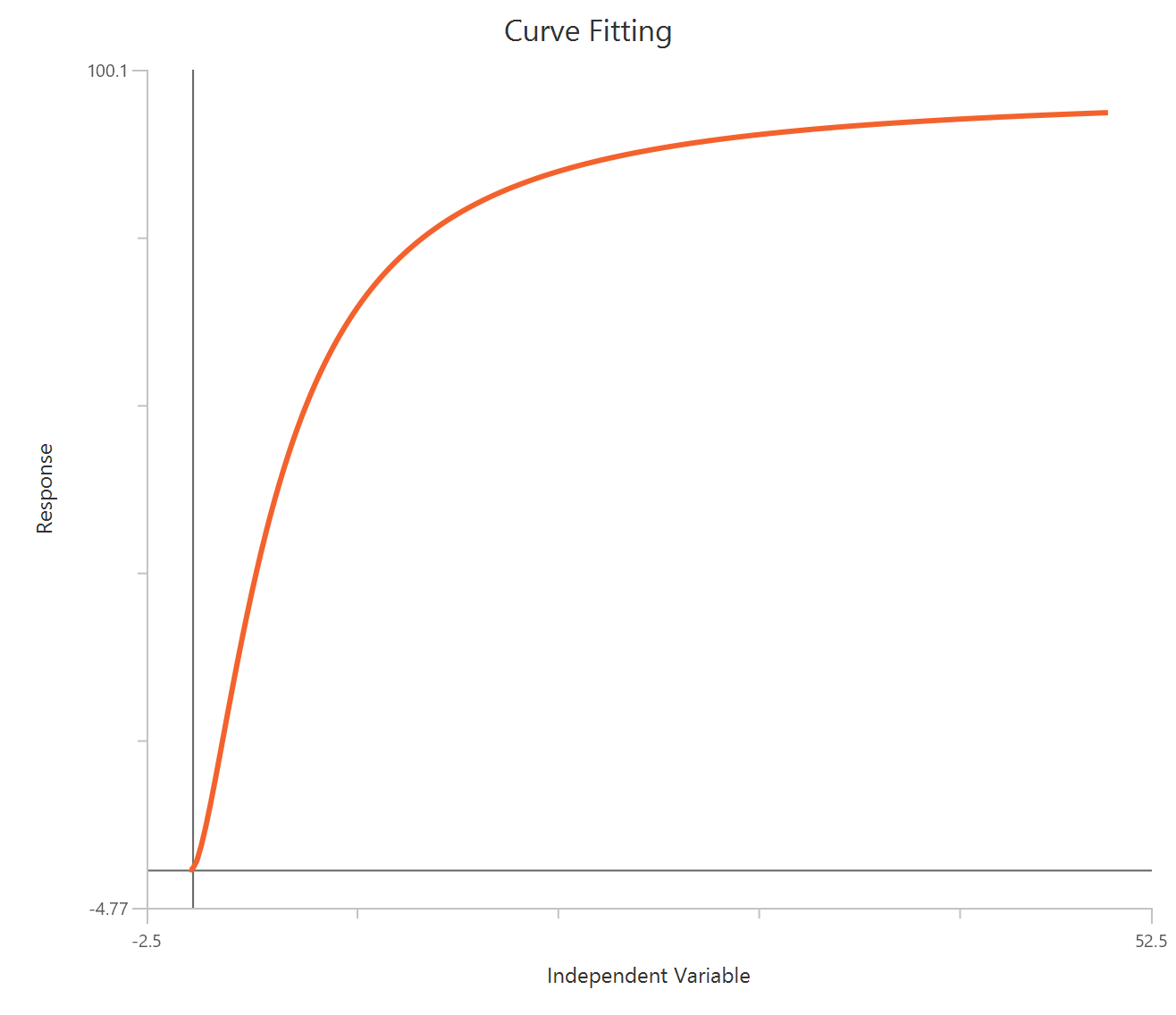
Input

The independent variable (X) must be on a linear scale and therefore must be strictly positive \((X>0)\). Zero or negative X values are not used in the calculations (they are ignored/excluded). The dependent variable (\(Y\)) should contain specific binding values in consistent units, with any nonspecific binding removed prior to fitting.

Parameters

1. \(Bmax\): The maximum specific binding capacity of the high-affinity site population (plateau contribution from that site). Reported in the same units as \(Y\).

2. \(K_d\): The concentration scale parameter in the same units as \(X\). When \(h=1\), \(K_d\) is the equilibrium dissociation constant and equals the ligand concentration that yields half-maximal specific binding. When \(h \neq 1\), \(K_d\) still sets the concentration range where the curve transitions, but its strict mechanistic interpretation as a true dissociation constant depends on why \(h\) differs from 1.

3. \(h\): Controls the steepness of the binding curve:

   1. \(h=1\): classic one-site binding (no cooperativity)
   2. \(h>1\): steeper, more sigmoidal transition (often associated with positive cooperativity or multiple interacting sites)
   3. \(0<h<1\): shallower transition (often consistent with site heterogeneity or negative cooperativity)

---

One site - Fit Ki, X is log10(competitor)

The One site — Fit Ki model is used in competition binding experiments to estimate the affinity (\(K_i\)) of an unlabeled competitor ligand. Binding of a fixed concentration of radioligand is measured while increasing concentrations of the competitor are added. As competitor concentration increases, radioligand binding decreases in a sigmoidal manner when plotted versus the log10 competitor concentration. The model fits this inhibition curve and converts the fitted midpoint to \(K_i\) using the Cheng–Prusoff relationship, accounting for the radioligand concentration and its \(K_d\).

Equation

\[ \begin{equation} \begin{alignedat}{2} \mathrm{LogEC50} &= \log_{10}\!\Big(10^{\mathrm{log}K_i}\big(1+\frac{\mathrm{HotNM}}{\mathrm{HotKdNM}}\big)\Big) \qquad & \\ Y &= \mathrm{Bottom} + \frac{\mathrm{Top}-\mathrm{Bottom}}{1+10^{(X-\mathrm{LogEC50})}} \qquad & \end{alignedat} \end{equation} \]

Visualization

Input

The independent variable (X) must be the log10-transformed competitor concentration (i.e., \(𝑋 = log_{10}(competitor)\)). The model also requires a column containing the dependent variable (Y) response values (in any consistent units). This equation also requires the specification of two extra parameters:

1. \(HotNM\): The concentration of radioligand used in the experiment (in nM). It is constant across the dataset.

2. \(HotKdNM\): The equilibrium dissociation constant (\(K_d\)) of the radioligand (in nM). Used to convert the fitted midpoint to \(K_i\).

Parameters

1. \(Top\): The upper plateau of the curve (binding when competitor is very low/absent). Reported in the same units as \(Y\).

2. \(Bottom\): The lower plateau of the curve (residual binding at very high competitor concentrations). Reported in the same units as \(Y\).

3. \(logK_i\): The base-10 logarithm of the competitor affinity. It is the primary fitted affinity parameter reported on a log scale.

---

One site - Fit LogIC50, X is log10(competitor)

The One site — Fit Ki model is used in competition binding experiments to estimate the affinity (\(K_i\)) of an unlabeled competitor ligand. Binding of a fixed concentration of radioligand is measured while increasing concentrations of the competitor are added. As competitor concentration increases, radioligand binding decreases in a sigmoidal manner when plotted versus the log10 competitor concentration. The model fits this inhibition curve and converts the fitted midpoint to \(K_i\) using the Cheng–Prusoff relationship, accounting for the radioligand concentration and its \(K_d\).

Equation

\[ \begin{equation} \begin{alignedat}{2} Y &= \mathrm{Bottom} + \frac{\mathrm{Top}-\mathrm{Bottom}}{1+10^{(X-\mathrm{LogIC50})}} \qquad & \end{alignedat} \end{equation} \]

Visualization

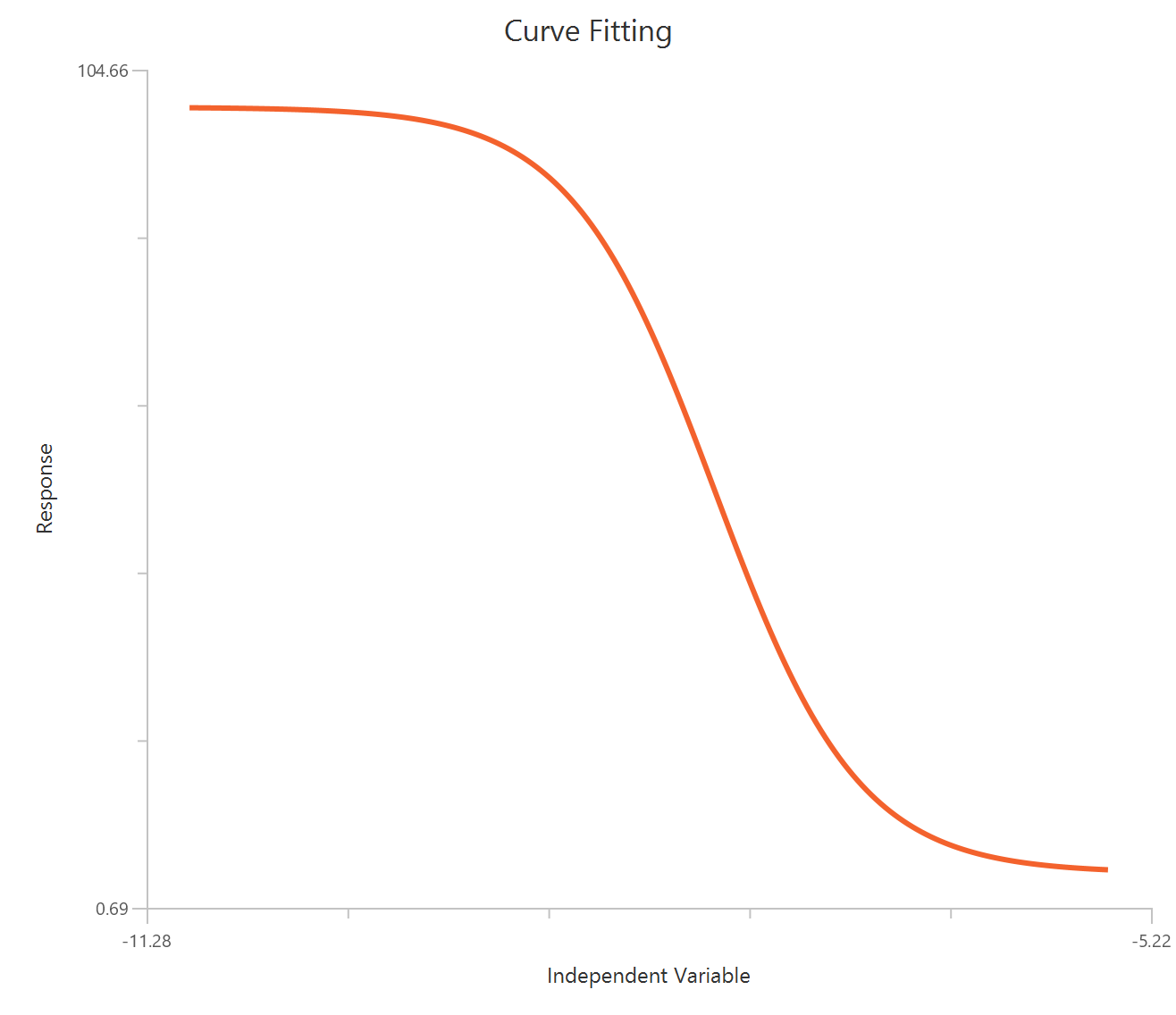
Input

The independent variable (X) must be the log10-transformed competitor concentration (i.e., \(𝑋 = log_{10}(competitor)\)). The model also requires a column containing the dependent variable (Y) response values (in any consistent units).

Parameters

1. \(Top\): The upper plateau of the curve (binding when competitor is very low/absent). Reported in the same units as \(Y\).

2. \(Bottom\): The lower plateau of the curve (residual binding at very high competitor concentrations). Reported in the same units as \(Y\).

3. \(LogIC50\): The base-10 logarithm of the competitor concentration that reduces binding to halfway between \(Top\) and \(Bottom\). Lower \(LogIC50\) (or \(IC50\)) values indicate higher competitor potency.

---

Two sites - Fit Ki, X is log10(competitor)

The Two sites — Fit Ki model is used in competition binding experiments when the radioligand (or receptor population) exhibits two binding site classes (typically high- and low-affinity). Binding is measured at a fixed radioligand concentration while increasing concentrations of an unlabeled competitor are added, with \(X\) entered as the log10 competitor concentration. The curve is fit as the sum of two sigmoidal inhibition components, weighted by the fraction of sites in the high-affinity class. The fitted midpoints are converted to two \(K_i\) values (high and low) using a Cheng–Prusoff–style adjustment that accounts for radioligand concentration and the radioligand \(K_d\) for each site class.

Equation

\[ \begin{equation} \begin{alignedat}{2} \mathrm{LogEC50}_{\mathrm{Lo}} &= \log_{10}\!\Big(10^{\mathrm{log}K_{i,\mathrm{Lo}}}\big(1+\frac{\mathrm{HotNM}}{\mathrm{HotKdNM}_{\mathrm{Lo}}}\big)\Big) \qquad & \mathrm{LogEC50}_{\mathrm{Hi}} &= \log_{10}\!\Big(10^{\mathrm{log}K_{i,\mathrm{Hi}}}\big(1+\frac{\mathrm{HotNM}}{\mathrm{HotKdNM}_{\mathrm{Hi}}}\big)\Big) \\ \mathrm{Span} &= \mathrm{Top}-\mathrm{Bottom} \qquad & \mathrm{Part}_1 &= \frac{\mathrm{FractionHi}\cdot \mathrm{Span}}{1+10^{(X-\mathrm{LogEC50}_{\mathrm{Hi}})}} \\ \mathrm{Part}_2 &= \frac{(1-\mathrm{FractionHi})\cdot \mathrm{Span}}{1+10^{(X-\mathrm{LogEC50}_{\mathrm{Lo}})}} \qquad & \end{alignedat} \end{equation} \]

\[ \begin{equation} Y=\mathrm{Bottom}+\mathrm{Part}_1+\mathrm{Part}_2 \end{equation} \]

Visualization

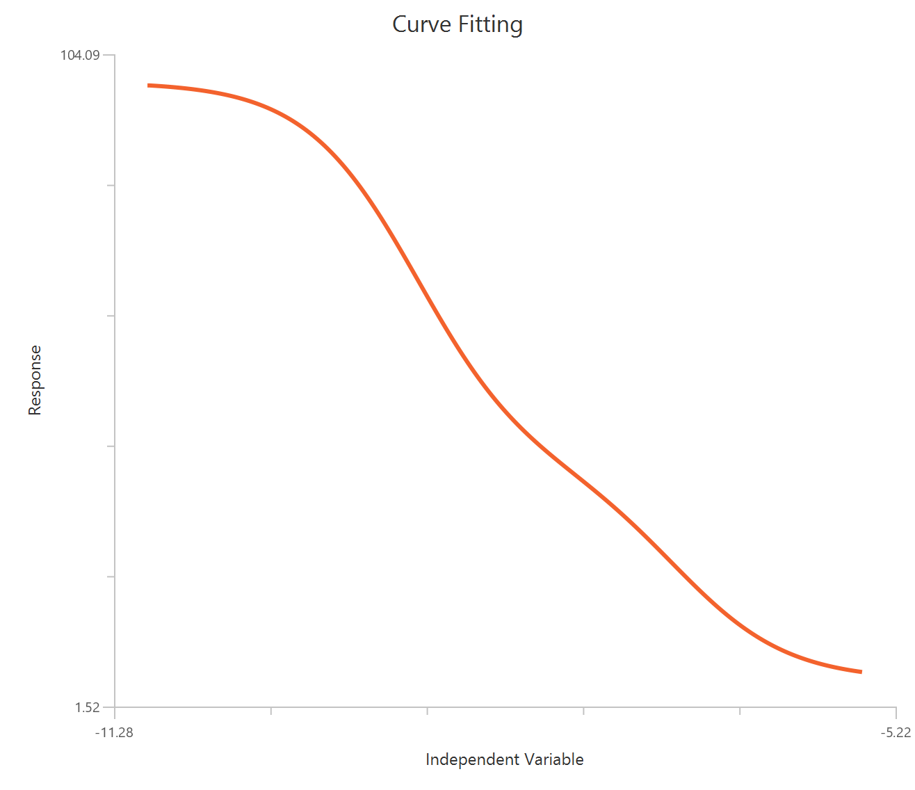
Input

The independent variable (X) must be the log10-transformed competitor concentration (i.e., \(𝑋 = log_{10}(competitor)\)). The model also requires a column containing the dependent variable (Y) response values (in any consistent units). This equation also requires the specification of three extra parameters:

1. \(HotNM\): Radioligand concentration used in the experiment (nM), constant across the dataset.

2. \(HotKdNM_{Hi},HotKdNM_{Lo}\): Radioligand \(K_d\) values (nM) for the high- and low-affinity site classes. Used in the Cheng–Prusoff adjustment that links \(IC50\) midpoints to \(K_i\).

Parameters

1. \(Top\): The upper plateau of the curve (binding when competitor is very low/absent). Reported in the same units as \(Y\).

2. \(Bottom\): The lower plateau of the curve (residual binding at very high competitor concentrations). Reported in the same units as \(Y\).

3. \(FractionHi\): The fraction of binding sites (or binding component) that follow the high-affinity competitor interaction. Constrained to \(0≤FractionHi≤1\). The low-affinity fraction is \(1−FractionHi\).

4. \(logK_i^{Hi}, logK_i^{Lo}\): Base-10 logarithms of the competitor affinities for the high- and low-affinity site classes.

---

Two sites - Fit LogIC50, X is log10(competitor)

The Two sites — Fit logIC50 model is used for competition binding experiments when the data suggest two distinct classes of binding sites (or binding components) with different affinities for the competitor. Binding is measured at a fixed radioligand concentration while increasing concentrations of unlabeled competitor are added, with \(X\) entered as the log₁₀ competitor concentration. The observed inhibition curve is modeled as the sum of two logistic components, each with its own midpoint (logIC50), weighted by the fraction of sites belonging to the high-affinity class. Unlike the “Fit Ki” version, this model does not convert midpoints to \(K_i\); instead, it directly estimates two empirical logIC50 values that describe where each component is half-inhibited.

Equation

\[ \begin{equation} \begin{alignedat}{2} \mathrm{Span} &= \mathrm{Top}-\mathrm{Bottom} \qquad & \\ \mathrm{Part}_1 &= \frac{\mathrm{FractionHi}\cdot \mathrm{Span}} {1+10^{(X-\mathrm{LogIC50}_{\mathrm{Hi}})}} \qquad & \mathrm{Part}_2 = \frac{(1-\mathrm{FractionHi})\cdot \mathrm{Span}} {1+10^{(X-\mathrm{LogIC50}_{\mathrm{Lo}})}} \end{alignedat} \end{equation} \]

\[ \begin{equation} Y = \mathrm{Bottom} + \mathrm{Part}_1 + \mathrm{Part}_2 \end{equation} \]

Visualization

Input

The independent variable (X) must be the log10-transformed competitor concentration (i.e., \(𝑋 = log_{10}(competitor)\)). The model also requires a column containing the dependent variable (Y) response values (in any consistent units).

Parameters

1. \(Top\): The upper plateau of the curve (binding when competitor is very low/absent). Reported in the same units as \(Y\).

2. \(Bottom\): The lower plateau of the curve (residual binding at very high competitor concentrations). Reported in the same units as \(Y\).

3. \(FractionHi\): The fraction of binding sites (or binding component) that follow the high-affinity competitor interaction. Constrained to \(0≤FractionHi≤1\). The low-affinity fraction is \(1−FractionHi\).

4. \(LogIC50_{Hi}, LogIC50_{Lo}\): Base-10 logarithms of the \(log_{10}(concentration)\) that inhibits half of the high/low-affinity component.

---

One site - Homologous

The One site — Homologous model is used in competition binding experiments where the labeled and unlabeled ligands are assumed to have identical affinity for the same single class of receptors (i.e., they are chemically identical or behave equivalently at the binding site). Binding of a fixed concentration of radioligand is measured while increasing concentrations of the unlabeled (cold) ligand are added, with \(X\) entered as the \(log_{10}\) competitor concentration. Because both ligands are assumed to share the same \(K_d\), the analysis allows you to estimate a single common affinity along with Bmax and a linear nonspecific component.

Equation

\[ \begin{equation} \begin{alignedat}{2} \mathrm{ColdNM} &= 10^{X} \qquad \text{(cold competitor in nM)} \\ \mathrm{KdNM} &= 10^{\mathrm{LogKd}} \qquad \text{(shared affinity in nM)} \end{alignedat} \end{equation} \]

\[ \begin{equation} Y = \frac{\mathrm{Bmax}\cdot \mathrm{HotNM}} {\mathrm{HotNM}+\mathrm{ColdNM}+\mathrm{KdNM}} + \mathrm{Bottom} \end{equation} \]

(Here HotNM is the fixed radioligand concentration for a given curve, and ColdNM is the competitor concentration derived from \(X=log_{10}(competitor)\).)

Visualization

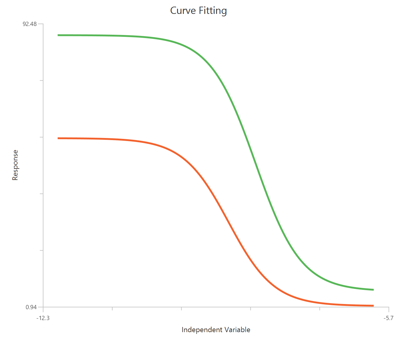
Input

The independent variable (X) must be the log10-transformed competitor concentration (i.e., \(𝑋 = log_{10}(competitor)\)). The model also requires at lease one column containing the dependent variable (Y) response values (in any consistent units). You must provide the radioligand concentration (HotNM) for each curve. Using at least two different radioligand concentrations is recommended for more reliable estimation of \(K_d, Bmax\), and nonspecific binding.

Parameters

1. \(LogKd\): The base-10 logarithm of the equilibrium dissociation constant shared by both labeled and unlabeled ligand.

2. \(Bmax\): The maximum binding capacity of the receptor system (same units as \(Y\)). It represents binding when receptors are saturated with ligand.

3. \(NS\): A constant baseline representing nonspecific binding (or residual signal). It is effectively the binding observed at very high competitor concentrations and is reported in the same units as \(Y\). Conceptually, this reflects the fraction of radioligand that binds nonspecifically rather than to receptors.

---

One Site – Heterologous with depletion

The One Site — Heterologous with depletion model is used for competition binding experiments when a substantial fraction of the added radioligand becomes bound, so the free radioligand concentration is meaningfully lower than the amount added (ligand depletion). In this setting, the usual competition model (which assumes free ≈ added) can bias affinity estimates. This depletion-aware formulation uses the experimental design constants (radioligand amount in CPM, radioligand \(K_d\), specific activity, and reaction volume) to correct for depletion and fit the competition curve accordingly.Because the method relies on comparing added ligand and bound ligand in the same CPM units, it is intended for radioactive ligands and is generally not applicable to fluorescent ligand formats.

Equation

\[ \begin{equation} \begin{alignedat}{2} \mathrm{KdCPM} &= \mathrm{KdNM}\cdot \mathrm{SpAct}\cdot \mathrm{Vol}\cdot 1000 \qquad & \\ R &= \mathrm{NS}+1 \qquad & S &= 1+10^{(X-\mathrm{Log}K_i)}\cdot \mathrm{KdCPM} + \mathrm{Hot} \\ a &= -1\cdot R \qquad & b &= R\cdot S + R\cdot \mathrm{Hot} + \mathrm{Bmax} \\ c &= -1\cdot \mathrm{Hot}\,(S\cdot \mathrm{NS} + \mathrm{Bmax}) \qquad & \end{alignedat} \end{equation} \]

\[ \begin{equation} Y=\frac{-b+\sqrt{b^{2}-4ac}}{2a} \end{equation} \]

Visualization

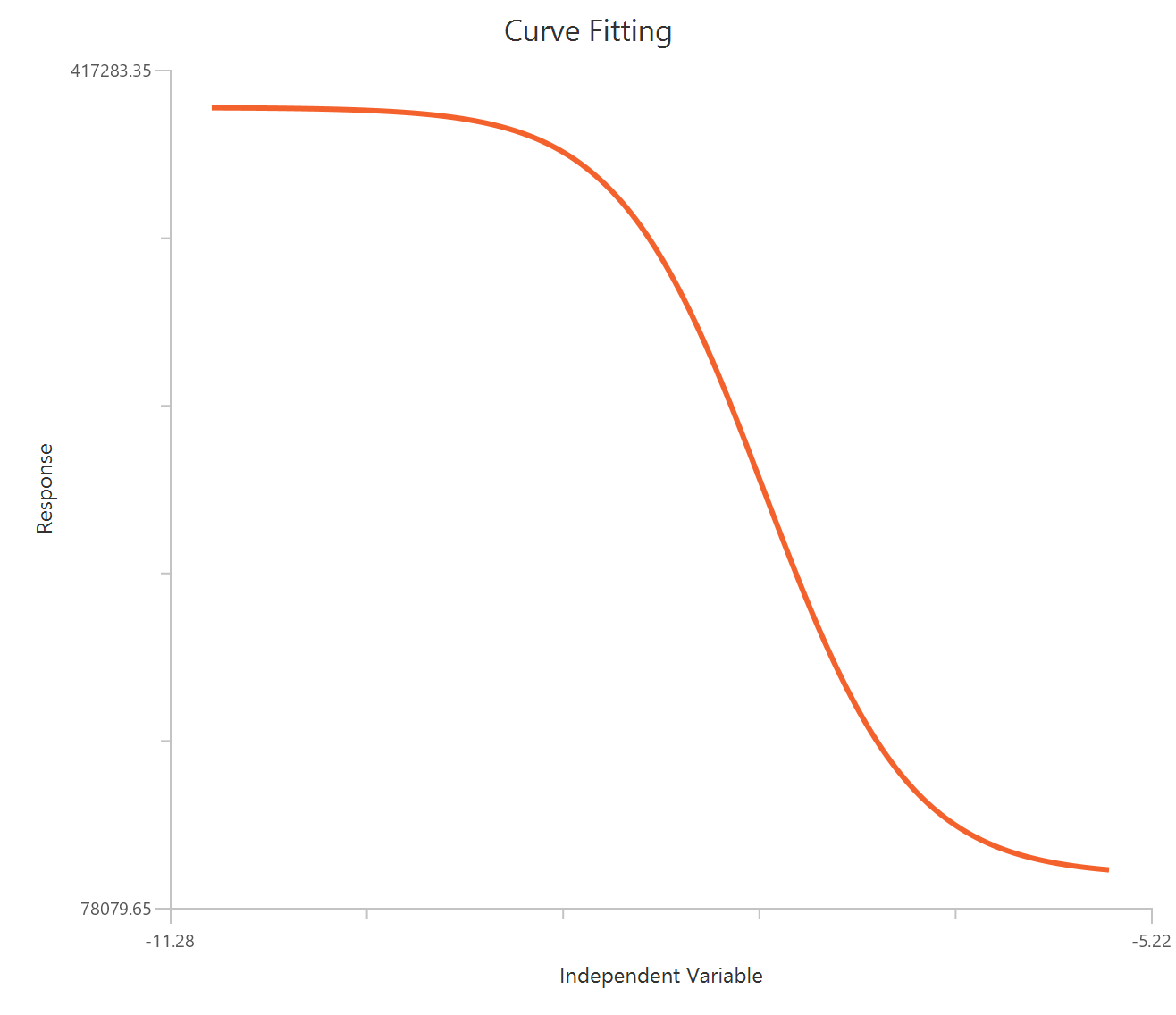
Input

The independent variable (X) must be the log10-transformed competitor concentration (i.e., \(𝑋 = log_{10}(competitor)\)). The model also requires a column containing the dependent variable (Y) response values (in any consistent units). This equation also requires the specification of three extra parameters:

1. \(Hot\): The amount/concentration of radioligand used for the experiment, expressed in CPM (constant across the dataset).

2. \(KdNM\): The radioligand equilibrium dissociation constant in nM.

3. \(SpAct\): Specific radioactivity (e.g., CPM per fmol), used to convert concentration units into CPM units.

4. \(Vol\): Reaction volume (e.g., mL), used in the concentration → CPM conversion for \(KdCPM\).

Parameters

1. \(LogKi\): The base-10 logarithm of the competitor affinity.

2. \(Bmax\): The maximum specific binding capacity (in CPM) corresponding to saturable receptor binding. Because it represents total receptor capacity, it is typically higher than the observed “Top” of an inhibition curve.

3. \(NS\): The nonspecific binding fraction (or proportionality factor) describing the portion of radioligand signal attributable to nonspecific binding sites under this CPM-based formulation.

---

Dissociation Kinetics

The Dissociation kinetics model describes how receptor–ligand binding decreases over time after conditions are changed to prevent re-binding (e.g., by adding excess unlabeled ligand, washing away radioligand, or strong dilution). Under the assumption of a single dominant dissociation process, the bound complex decays as a one-phase exponential, approaching a constant residual level at long times. The fitted dissociation rate constant (\(k_{off}\)) quantifies how quickly ligand dissociates from the receptor.

Equation

\[ \begin{equation} \begin{alignedat}{2} Y &= (Y_0-\mathrm{NS})\,e^{-k_{\mathrm{off}}X} + \mathrm{NS} \qquad & \end{alignedat} \end{equation} \]

Visualization

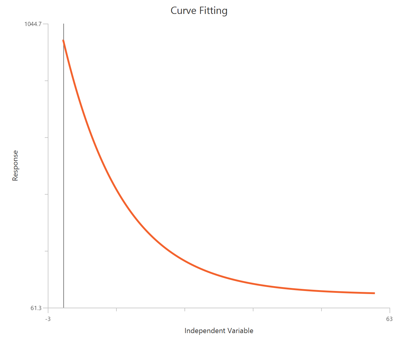
Input

The independent variable (X) must be on a linear scale and therefore must be strictly positive \((X>0)\). Zero or negative X values are not used in the calculations (they are ignored/excluded). The dependent variable (\(Y\)) is the measured binding signal (total or specific, depending on your assay) in consistent units.

Parameters

1. \(Y_0\): Binding at time zero (immediately after initiating dissociation), in the same units as \(Υ\).

2. \(NS\): The asymptotic binding at very long times (the plateau the curve approaches). This is often interpreted as residual nonspecific binding or incomplete dissociation, in the same units as \(Υ\).

3. \(k_{off}\): (must be positive) The dissociation rate constant (units of 1/time). Larger \(k_{off}\) means faster dissociation. The dissociation half-life is:

\[ \begin{equation} \begin{alignedat}{2} t_{1/2} &= \frac{ln(2)}{k_{off}} \qquad & \end{alignedat} \end{equation} \]

---

Association Kinetics – One Ligand

The Association kinetics (one ligand concentration) model describes how radioligand binding increases over time toward equilibrium at a single fixed ligand concentration. The time course follows a single exponential approach to a maximum, governed by an apparent rate constant that depends on both association and dissociation. In this formulation, you fix the dissociation rate constant (koff) from an independent experiment and estimate the association rate constant (kon) from the binding time course. This model assumes a simple one-site binding process with no ligand depletion and constant ligand concentration throughout the experiment.

Equation

\[ \begin{equation} \begin{aligned} K_d &= \frac{k_{\text{off}}}{k_{\text{on}}} \\ [L] &= \mathrm{HotNm}\cdot 10^{-9} \\ k_{\text{obs}} &= k_{\text{on}}\,[L] + k_{\text{off}} \\ \mathrm{Occupancy} &= \frac{[L]}{[L]+K_d} \\ Y_{\max} &= \mathrm{Occupancy}\cdot B_{max} \\ Y(t) &= Y_{\max}\left(1-e^{-k_{\text{obs}}\, t}\right) \end{aligned} \end{equation} \]

Visualization

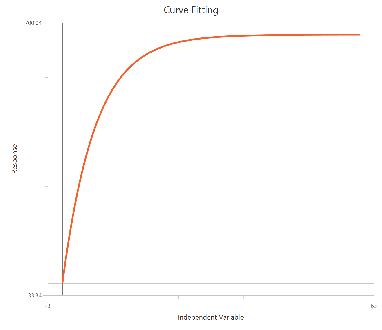
Input

The independent variable (X) must be time on a linear scale and therefore must be non-negative (\(X≥0\)). The model also requires a column containing the dependent variable (Y) response values (in any consistent units). This equation also requires the specification of three extra parameters:

1. \(Hotnm\): The radioligand concentration in nM (a single concentration is used for the entire experiment).

2. \(k_{off}\): the dissociation rate constant in \(min^{-1}\) (must be positive).

Parameters

1. \(k_{on}\): Association rate constant, in \(min^{-1}\). Describes how rapidly ligand binds to free receptors.

2. \(Bmax\): The maximal binding at equilibrium (same units as \(Y\)), extrapolated to maximal radioligand concentration.

---

Association Kinetics – Two or More Ligand Concentrations

This model describes radioligand association measured at two or more fixed ligand concentrations, which allows simultaneous estimation of both \(k_{on}\) and \(k_{off}\) from a single global fit. Because the observed association rate depends on both rate constants and ligand concentration, fitting multiple concentrations removes the ambiguity that exists when only one concentration is used. All time courses are assumed to follow a single-exponential approach to equilibrium with a concentration-dependent observed rate constant.

Equation

\[ \begin{equation} \begin{aligned} K_d &= \frac{k_{\text{off}}}{k_{\text{on}}} \\[4pt] [L] &= \mathrm{HotNm}\cdot 10^{-9} \\[4pt] k_{\text{obs}} &= k_{\text{on}}\,[L] + k_{\text{off}} \\[4pt] \mathrm{Occupancy} &= \frac{[L]}{[L]+K_d} \\[4pt] Y_{\max} &= \mathrm{Occupancy}\cdot B_{max} \\[4pt] Y(t) &= Y_{\max}\left(1-e^{-k_{\text{obs}}\, t}\right) \end{aligned} \end{equation} \]

Visualization

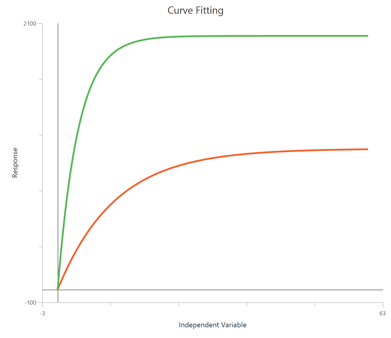
Input

The independent variable (X) must be time on a linear scale and therefore must be non-negative (\(X≥0\)). The model also requires at lease one column containing the dependent variable (Y) response values (in any consistent units). You must provide the radioligand concentration (HotNM) for each curve.

Parameters

1. \(k_{on}\): Association rate constant, in \(min^{-1}\).

2. \(k_{off}\): Dissociation rate constant, in \(min^{-1}\).

3. \(Bmax\): The maximal binding at equilibrium (same units as \(Y\)), extrapolated to maximal radioligand concentration.

---

Association then Dissociation

The Association then dissociation model fits a single time-course experiment where binding is first allowed to associate toward equilibrium at a fixed radioligand concentration, and then at a defined time point (Time0) dissociation is initiated (e.g., by adding excess unlabeled ligand or performing a large dilution). The model combines an exponential association phase (governed by \(k_{on}\) and \(k_{off}\) through \(k_{obs}\)) with an exponential dissociation phase (governed by \(k_{off}\) alone). By fitting both phases in one dataset, the model can estimate \(k_{on}\) and \(k_{off}\) without requiring multiple ligand concentrations. The predicted response includes the parameter \(NS\) to capture nonspecific binding or baseline signal.

Equation

\[ \begin{equation} \begin{aligned} \mathrm{Radioligand} &= \mathrm{HotNM}\cdot 10^{-9} \\ k_{\text{obs}} &= \mathrm{Radioligand}\cdot k_{on} + k_{off} \\ K_d &= \frac{k_{off}}{k_{on}} \\ Eq &= B_{max}\cdot \frac{\mathrm{Radioligand}}{\mathrm{Radioligand}+K_d} \\ \mathrm{Association}(X) &= Eq\left(1-e^{-k_{\text{obs}}X}\right) \\ Y_{at\,Time0} &= Eq\left(1-e^{-k_{\text{obs}}\,Time0}\right) \\ \mathrm{Dissociation}(X) &= Y_{at\,Time0}\,e^{-k_{off}(X-Time0)} \\ Y &= \mathrm{IF}(X<Time0,\ \mathrm{Association}(X),\ \mathrm{Dissociation}(X)) + NS \end{aligned} \end{equation} \]

Visualization

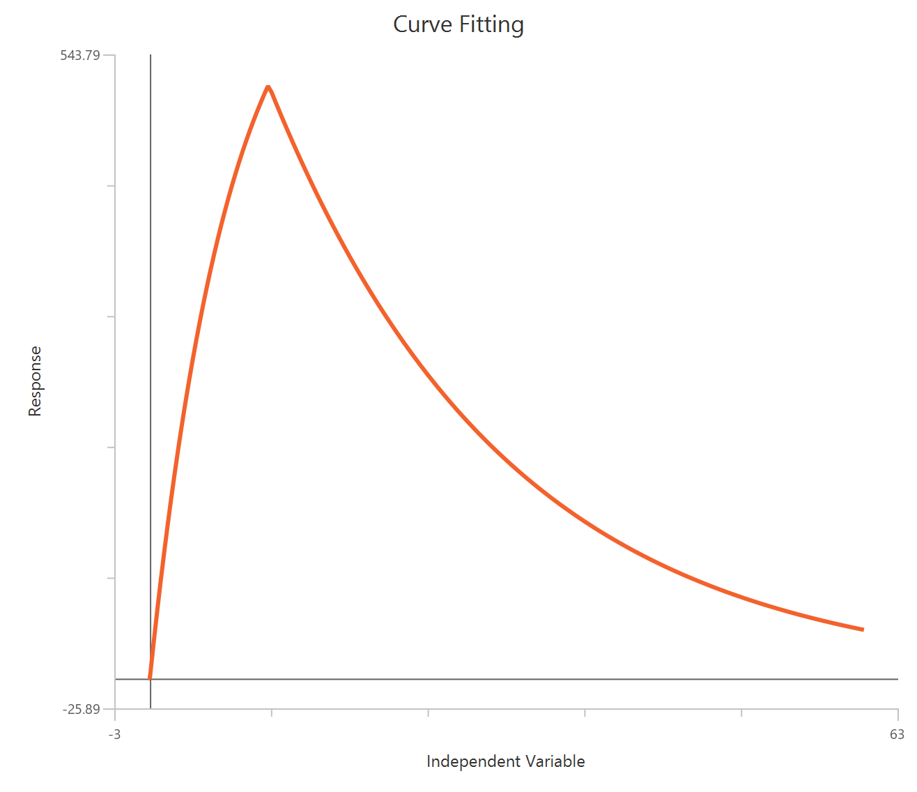
Input

The independent variable (X) must be time on a linear scale (e.g., minutes) and therefore must be non-negative (\(X≥0\)). The dependent variable (Y) must be binding measured in any consistent units. The model requires the specification of two extra parameters:

1. \(Hotnm\): The radioligand concentration in nM (a single concentration is used for the entire experiment).

2. \(Time of switch\)$: the time (in the same units as X) at which dissociation is initiated.

Parameters

1. \(k_{on}\): The association rate constant, in \(min^{-1}\) (or inverse time matching X). \(k_{off}\) must be strictly positive.

2. \(k_{off}\): The dissociation rate constant, in \(min^{-1}\) (or inverse time matching X). \(k_{off}\) must be strictly positive.

3. \(Bmax\): The maximal binding capacity (same units as \(Y\)), extrapolated to saturation.

4. \(NS\): The constant baseline (nonspecific binding/offset) in the units of \(Y\). It represents the binding level at \(X=0\) and the residual level approached at long times after dissociation.

---

Kinetics - Competitive Binding

The Kinetics of competitive binding model estimates the association and dissociation rate constants of an unlabeled competitor by measuring how the binding of a labeled radioligand changes over time when both ligands are added together. The kinetic parameters of the labeled ligand are treated as known (constrained from separate kinetic experiments), and the model fits the kinetic parameters of the unlabeled ligand by globally analyzing time courses collected at two or more competitor concentrations. Because the interaction between labeled and unlabeled ligands produces a biexponential time course, the model computes two observed rate constants and combines them to predict the time-dependent specific binding.

Equation

\[ \begin{equation} \begin{aligned} K_A &= k_1\cdot L \cdot 10^{-9} + k_2 \\ K_B &= k_3\cdot I \cdot 10^{-9} + k_4 \\ S &= \sqrt{(K_A-K_B)^2 + 4\,k_1k_3\,I\,L\cdot 10^{-18}} \\ K_F &= \frac{1}{2}\left(K_A+K_B+S\right) \\ K_S &= \frac{1}{2}\left(K_A+K_B-S\right) \\ DIFF &= K_F-K_S \\ Q &= \frac{B_{max}\,k_1\,I\cdot 10^{-9}}{DIFF} \\ Y &= Q\left(\frac{k_4\,DIFF}{K_FK_S} + \frac{K_4-K_F}{K_F}e^{-K_FX} - \frac{K_4-K_S}{K_S}e^{-K_SX}\right) \end{aligned} \end{equation} \]

Visualization

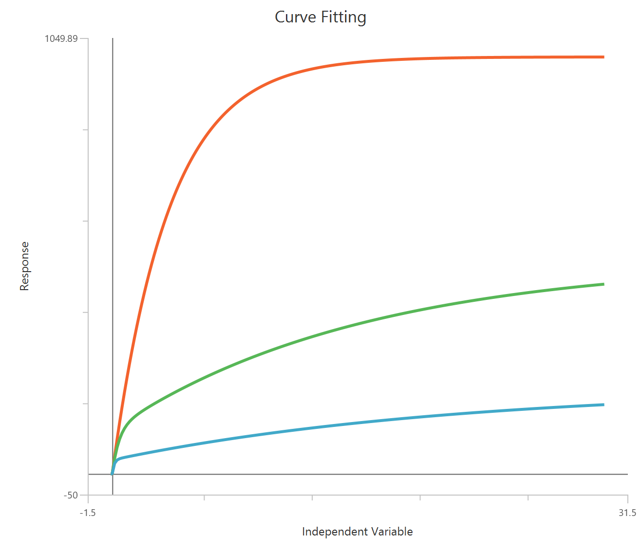
Input

The independent variable (X) must be time on a linear scale and therefore must be non-negative (\(X≥0\)). The model also requires at lease one column containing the dependent variable (Y) response values (in any consistent units). The unlabeled ligand concentrations (in nM) must be provided for each curve.The model requires the specification of three extra parameters:

1. \(k_1 (1/M*min)\): The association rate constant of the labeled ligand.

2. \(k_2 (1/min)\): The dissociation rate constant of the labeled ligand.

3. \(L (nM)\): The concentration of labeled ligand (radioligand) in nM, treated as constant for the experiment.

Parameters

1. \(k_3\): The association rate constant of the unlabeled ligand, in \((1/M*min)\). .

2. \(k_4\): Dissociation rate constant, in \(min^{-1}\).

3. \(Bmax\): The maximal binding capacity (same units as \(Y\)), representing total receptor binding capacity.

---

Enzyme Kinetics

Michaelis-Menten

The Michaelis–Menten model describes classic steady-state enzyme kinetics when substrate concentration is varied and initial reaction velocity is measured. The model assumes that enzyme–substrate complex formation reaches a quasi-steady state and that product formation is rate-limiting. As substrate concentration increases, velocity rises rapidly at low concentrations and then approaches an asymptotic maximum velocity (\(V_{max}\)). This formulation is appropriate when the concentration of enzyme catalytic sites is unknown or when the primary quantities of interest are (\(V_{max}\)) and (\(K_{m}\)) rather than (\(k_{cat}\)).

Equation

\[ \begin{equation} Y = \frac{V_{max}\, X}{K_m + X} \end{equation} \]

Visualization

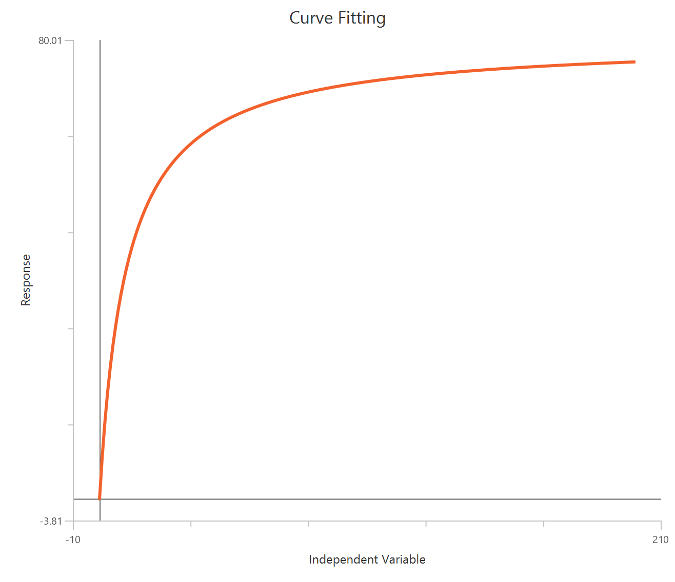
Input

The independent variable (X) must be substrate concentration on a linear scale and must be strictly positive (\(𝑋 > 0\)); zero or negative values are excluded from the fit. The dependent variable (Y) must be initial enzyme velocity expressed in consistent concentration-per-time units (e.g., µM/min, nM/s). No additional fixed parameters are required for this model.

Parameters

1. \(V_{max}\): The maximal enzyme velocity in the same units as \(Y\). This is the velocity the enzyme would reach at infinitely high substrate concentration and is typically higher than any measured velocity in the experiment.

2. \(K_m\): The Michaelis–Menten constant, in the same units as \(X\). It is the substrate concentration required to reach half of \(V_{max}\). A lower \(K_m\) indicates higher apparent affinity of the enzyme for the substrate.

---

Determine kcat

The Determine kcat model is a re-parameterized form of the Michaelis–Menten equation used when the concentration of enzyme catalytic sites (Et) is known. Instead of fitting Vmax, the model estimates the turnover number (kcat) — the number of substrate molecules converted to product per catalytic site per unit time. The model assumes classic steady-state Michaelis–Menten kinetics: velocity increases with substrate concentration and asymptotically approaches a maximum rate equal to \(E_t*k_{cat}\). This formulation is useful when comparing catalytic efficiency across enzymes or conditions because kcat is independent of enzyme concentration, whereas Vmax is not.

Equation

\[ \begin{equation} Y = \frac{E_t \cdot k_{cat}\, X}{K_m + X} \end{equation} \]

Visualization

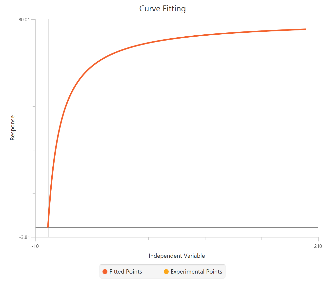
Input

The independent variable (X) must be substrate concentration on a linear scale and therefore must be strictly positive (\(X>0\)); zero or negative values are excluded. The dependent variable (Y) must be initial enzyme velocity in consistent concentration-per-time units (e.g., µM/min, nM/s). The model requires the specification of one extra parameter:

1. \(E_t\): the concentration of enzyme catalytic sites, in the same concentration units used for \(Y\) (time units are defined by kcat).

Parameters

1. \(k_{cat}\): The turnover number: the number of substrate molecules converted to product per catalytic site per unit time. Units are the inverse of the time units in \(Y\) (e.g., \(s^{-1}\) or \(min^{-1}\)). Larger \(k_{cat}\) means a faster enzyme.

2. \(K_m\): The Michaelis–Menten constant (same units as \(X\)). It is the substrate concentration required to reach half of the maximal velocity. Lower \(K_m\) indicates higher apparent affinity for substrate.

3. \(V_{max}\): The nonspecific binding fraction (or proportionality factor) describing the portion of radioligand signal attributable to nonspecific binding sites under this CPM-based formulation.

---

Allosteric (sigmoidal) enzyme kinetics

The Allosteric sigmoidal model describes enzyme kinetics when the enzyme displays cooperative substrate binding. In this case, the velocity–substrate curve is not hyperbolic (as in Michaelis–Menten) but sigmoidal. This behavior is captured empirically by adding a Hill coefficient to the Michaelis–Menten form. The model is useful when binding of substrate to one catalytic site alters the affinity of other sites, producing positive cooperativity.

Equation

\[ \begin{equation} Y = \frac{V_{max}\, X^h}{K_{half}^h + X^h} \end{equation} \]

Visualization

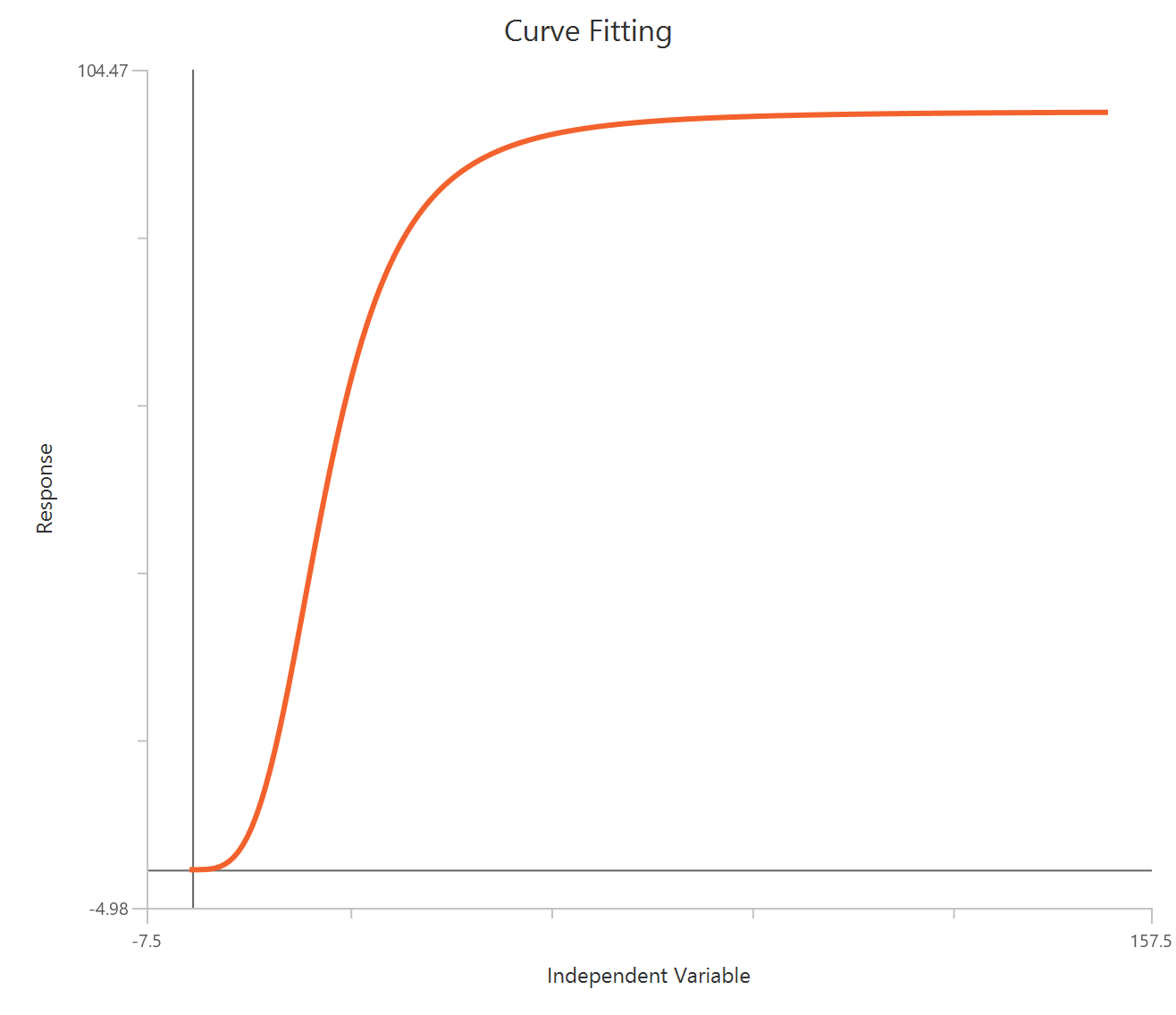
Input

The independent variable (X) must be substrate concentration on a linear scale and must be strictly positive (\(𝑋 > 0\)); zero or negative values are excluded from the fit. The dependent variable (Y) must be initial enzyme velocity expressed in consistent concentration-per-time units (e.g., µM/min, nM/s). No additional fixed parameters are required for this model.

Parameters

1. \(V_{max}\): The maximal enzyme velocity in the same units as \(Y\). This is the velocity the enzyme would reach at infinitely high substrate concentration and is typically higher than any measured velocity in the experiment.

2. \(K_{half}\): The substrate concentration that produces half-maximal velocity. It plays a role analogous to \(K_m\) in Michaelis–Menten kinetics and is sometimes called the EC50 for enzyme velocity.

3. \(h (Hill slope)\): An empirical measure of cooperativity and curve steepness. If:

   1. \(h=1\), the equation reduces to the standard Michaelis–Menten model.
   2. \(h>1\), the curve becomes sigmoidal, indicating positive cooperativity. h does not necessarily equal the number of binding sites; it reflects the degree of cooperative behavior rather than a strict mechanistic count.

---

Competitive Inhibition

The Competitive enzyme inhibition model describes enzyme kinetics in the presence of a reversible competitive inhibitor. A competitive inhibitor binds to the same active site as the substrate, so its effect can be overcome by increasing substrate concentration. As a result, \(V_{max}\) remains unchanged, while the apparent Michaelis–Menten constant increases. By fitting substrate–velocity curves measured at multiple inhibitor concentrations, the model estimates the inhibition constant \(K_i\) together with the shared kinetic parameters \(V_{max}\) and \(K_m\).

Equation

\[ \begin{equation} \begin{aligned} K_{m,obs} &= K_m\left(1+\frac{I}{K_i}\right) \\ Y &= \frac{V_{max}\,X}{K_{m,obs}+X} \end{aligned} \end{equation} \]

Visualization

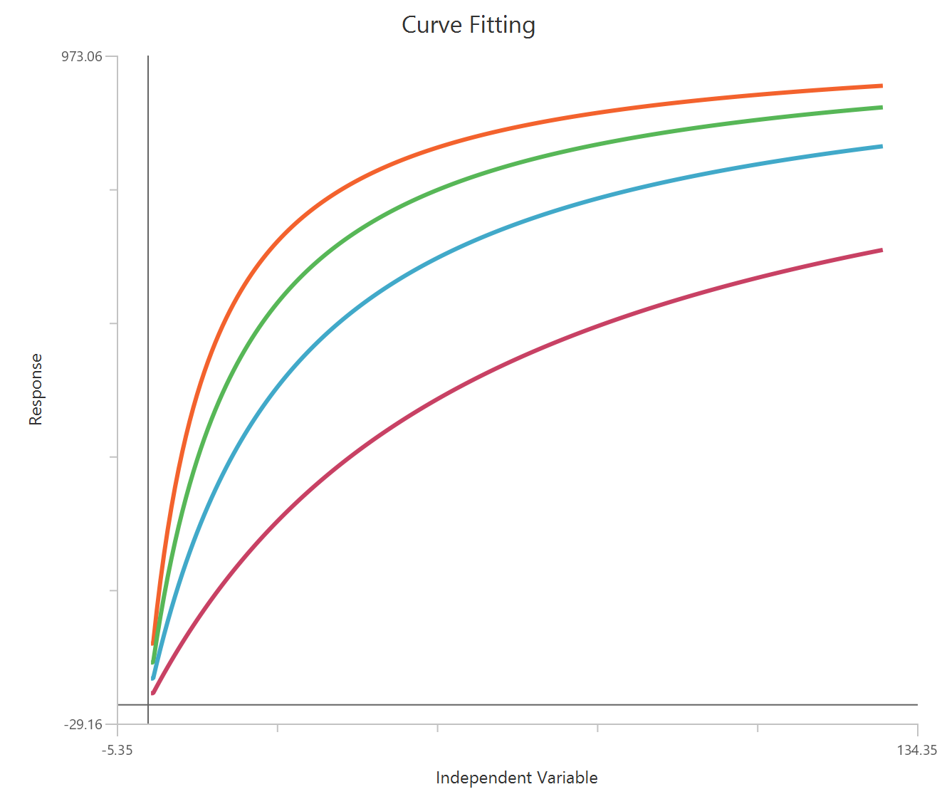
Input

The independent variable (X) must be substrate concentration on a linear scale and therefore must be strictly positive (\(X>0\)). The dependent variables (Y) must be enzyme velocity measured at several inhibitor concentrations. Each Y column represents one inhibitor concentration. The inhibitor concentration \(I\) (in the same units for all curves, typically µM) must be entered as numeric concentration values (not logarithms). These values are treated as data-set constants during fitting.

Parameters

1. \(V_{max}\): The maximal enzyme velocity in the absence of inhibitor, expressed in the same units as \(Y\). It is shared across all inhibitor concentrations.

2. \(K_{i}\): The inhibition constant, expressed in the same units as \(I\). It quantifies the affinity of the inhibitor for the enzyme. Lower \(K_i\) indicates stronger inhibition.

3. \(k_m\): The Michaelis–Menten constant in the absence of inhibitor, expressed in the same units as \(X\). It represents the substrate concentration required to reach half of \(𝑉_{max}\) when \(I=0\).

---

Noncompetitive Inhibition

The Noncompetitive enzyme inhibition model describes enzyme kinetics in the presence of an inhibitor that binds reversibly to both the free enzyme and the enzyme–substrate complex with the same affinity. In this simplified “pure noncompetitive” case, inhibition reduces the effective maximal velocity (\(V_{max}\)) while leaving \(K_m\) unchanged. By fitting substrate–velocity curves measured at multiple inhibitor concentrations, the model estimates the inhibition constant \(K_i\) together with the shared parameters \(V_{max}\) and \(K_m\). If inhibition does not follow this simplified behavior, a mixed-model inhibition equation is often more appropriate.

Equation

\[ \begin{equation} \begin{aligned} V_{max,inh} &= \frac{V_{max}}{1+\frac{I}{K_i}} \\ Y &= \frac{V_{max,inh}\,X}{K_m+X} \end{aligned} \end{equation} \]

Visualization

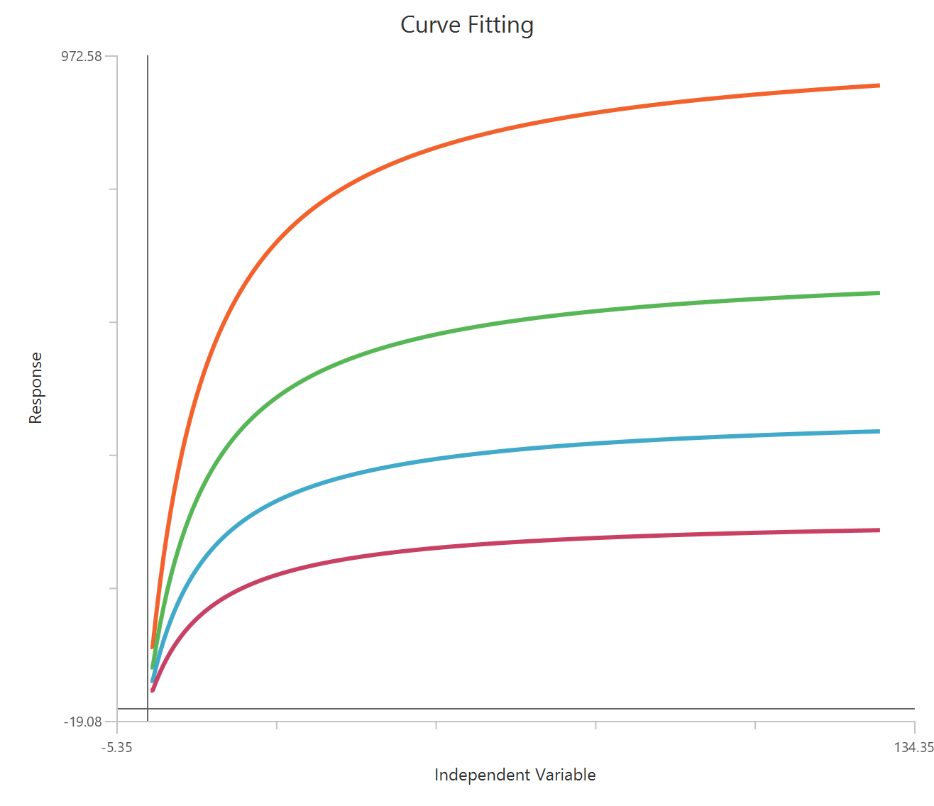
Input

The independent variable (X) must be substrate concentration on a linear scale and therefore must be strictly positive (\(X>0\)). The dependent variables (Y) must be enzyme velocity measured at multiple inhibitor concentrations. Each Y column represents one inhibitor concentration. The inhibitor concentration \(I\) (in the same units for all curves, typically µM) must be entered as numeric concentration values (not logarithms). These values are treated as data-set constants during fitting.

Parameters

1. \(V_{max}\): The maximum enzyme velocity in the absence of inhibitor, expressed in the same units as \(Y\). It is shared across all inhibitor concentrations.

2. \(K_{i}\): The inhibition constant, expressed in the same units as \(I\). It quantifies the affinity of the inhibitor for the enzyme. Lower \(K_i\) indicates stronger inhibition.

3. \(k_m\): The Michaelis–Menten constant in the absence of inhibitor, expressed in the same units as \(X\). It represents the substrate concentration required to reach half of \(𝑉_{max}\) when \(I=0\).

---

Uncompetitive Inhibition

The Uncompetitive enzyme inhibition model describes inhibition in which the inhibitor binds exclusively to the enzyme–substrate complex, not to the free enzyme. As a result, both the apparent maximal velocity and the apparent Michaelis constant decrease by the same factor. The substrate–velocity curves shift downward and to the left as inhibitor concentration increases. By fitting multiple curves measured at different inhibitor concentrations, the model estimates the inhibition constant together with the shared kinetic parameters of the uninhibited system.

Equation

\[ \begin{equation} \begin{aligned} V_{max}^{app} &= \frac{V_{max}}{1+\frac{I}{\alpha K_i}} \\ K_m^{app} &= \frac{K_m}{1+\frac{I}{\alpha K_i}} \\ Y &= \frac{V_{max}^{app}\,X}{K_m^{app}+X} \end{aligned} \end{equation} \]

Visualization

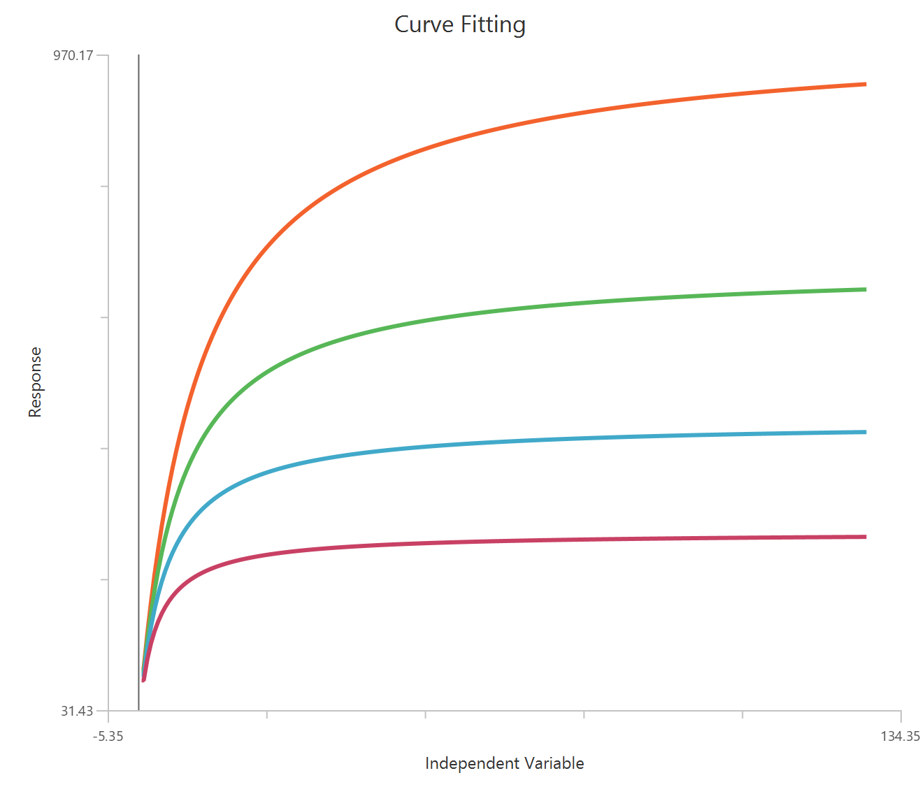
Input

The independent variable (X) must be substrate concentration on a linear scale and therefore must be strictly positive (\(X>0\)). The dependent variables (Y) must be enzyme velocity measured at several inhibitor concentrations. Each Y column represents one inhibitor concentration. The inhibitor concentration \(I\) (in the same units for all curves, typically µM) must be entered as numeric concentration values (not logarithms). These values are treated as data-set constants during fitting.

Parameters

1. \(V_{max}\): The maximal enzyme velocity in the absence of inhibitor, expressed in the same units as \(Y\). This parameter is shared across all inhibitor concentrations.

2. \(aK_{i}\): The effective inhibition constant for binding to the enzyme–substrate complex, expressed in the same units as \(I\). Only the product \(αK_i\) can be identified in this formulation.

3. \(k_m\): The Michaelis–Menten constant in the absence of inhibitor, expressed in the same units as \(X\). It represents the substrate concentration required to reach half of \(𝑉_{max}\) when \(I=0\).

---

Mixed-model Inhibition

The Mixed-model enzyme inhibition equation is the most general reversible inhibition model. It includes competitive, uncompetitive, and noncompetitive inhibition as special cases. In this framework, the inhibitor can bind both to the free enzyme and to the enzyme–substrate complex, but with potentially different affinities. The additional parameter \(α\) quantifies the relative preference of inhibitor binding to these two forms and therefore provides mechanistic insight into the mode of inhibition. By fitting multiple substrate–velocity curves measured at different inhibitor concentrations, the model estimates a single shared set of kinetic and inhibition parameters.

Equation

\[ \begin{equation} \begin{aligned} V_{max}^{app} &= \frac{V_{max}}{1+\frac{I}{\alpha K_i}} \\ K_m^{app} &= K_m \frac{1+\frac{I}{K_i}}{1+\frac{I}{\alpha K_i}} \\ Y &= \frac{V_{max}^{app}\,X}{K_m^{app}+X} \end{aligned} \end{equation} \]

Visualization

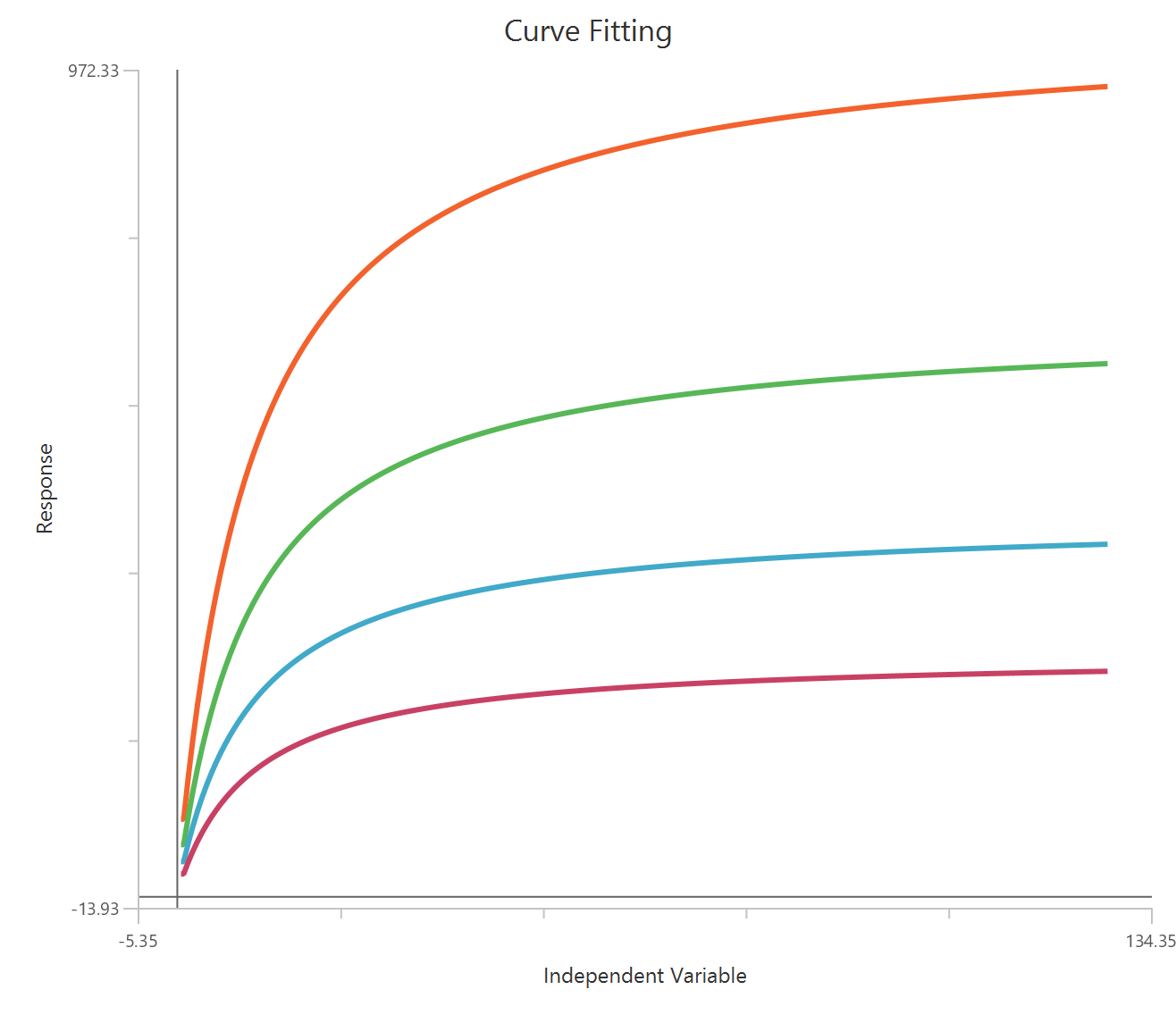
Input

The independent variable (X) must be substrate concentration on a linear scale and therefore must be strictly positive (\(X>0\)). The dependent variables (Y) must be enzyme velocity measured at several inhibitor concentrations. Each Y column represents one inhibitor concentration. The inhibitor concentration \(I\) (in the same units for all curves, typically µM) must be entered as numeric concentration values (not logarithms). These values are treated as data-set constants during fitting.

Parameters

1. \(V_{max}\): The maximal enzyme velocity in the absence of inhibitor, expressed in the same units as \(Y\). Shared across all inhibitor concentrations.

2. \(K_m\): The Michaelis–Menten constant in the absence of inhibitor, expressed in the same units as \(𝑋\).

3. \(K_i\): The inhibition constant for inhibitor binding to the free enzyme, expressed in the same units as \(I\).​

4. \(a\): The interaction factor describing how inhibitor binding affects substrate binding affinity. It is dimensionless and must be greater than zero.

   1. If \(α=1\), the inhibitor binds equally well to free enzyme and enzyme–substrate complex (pure noncompetitive inhibition).
   2. If \(α>1\), the inhibitor preferentially binds to the free enzyme (approaching competitive inhibition as \(α→∞\)).
   3. If \(α<1\) (but >0), the inhibitor preferentially binds to the enzyme–substrate complex (approaching uncompetitive inhibition as \(α→0\)).

---

Substrate Inhibition

The Substrate inhibition model describes enzyme kinetics in which high substrate concentrations reduce enzyme activity. This occurs when a second substrate molecule binds to the enzyme–substrate complex, forming an inactive ternary complex. As a result, velocity initially increases with substrate concentration following Michaelis–Menten behavior, reaches a maximum, and then decreases at higher substrate levels. This model is appropriate when the rate–substrate curve shows a clear peak followed by a decline.

Equation

\[ \begin{equation} Y = \frac{V_{max}\,X}{K_m + X\left(1+\frac{X}{K_i}\right)} \end{equation} \]

Visualization

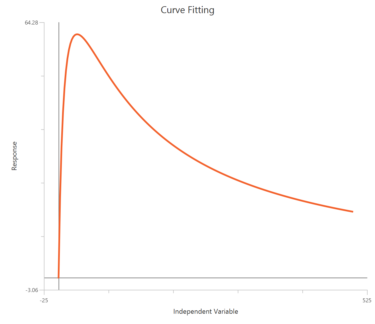
Input

The independent variable (X) must be substrate concentration on a linear scale and strictly positive (\(X>0\)). Zero or negative substrate concentrations are excluded. The dependent variable (Y) must be enzyme velocity measured in consistent concentration-per-time units (e.g., µM/min, nM/s).

Parameters

1. \(V_{max}\): The theoretical maximum enzyme velocity in the absence of substrate inhibition. Expressed in the same units as \(Y\).

2. \(K_m\): The Michaelis–Menten constant (same units as \(X\)). It is the substrate concentration at which velocity reaches half of \(V_{max}\) when substrate inhibition is negligible.

3. \(K_i\): The inhibition constant for binding of the second substrate molecule (same units as \(X\)). Smaller \(K_i\) values indicate stronger substrate inhibition (the decline in velocity begins at lower substrate concentrations).

---

Tight inhibition (Morrison equation)

The Tight inhibition model (Morrison equation) describes enzyme inhibition under conditions where the inhibitor binds with high affinity and its concentration is comparable to the enzyme concentration. In this regime, the free inhibitor concentration cannot be approximated by the total inhibitor concentration because a substantial fraction becomes bound to enzyme. This model explicitly accounts for ligand depletion and is appropriate when \([I] \sim [E]\) or when the inhibition curve deviates from standard Michaelis–Menten competitive behavior. Unlike classical inhibition models, this formulation requires independent knowledge of enzyme concentration and substrate conditions, as these cannot be reliably estimated from inhibition data alone.

Equation

\[ \begin{equation} Q = K_i\left(1+\frac{S}{K_m}\right) \end{equation} \]

Visualization

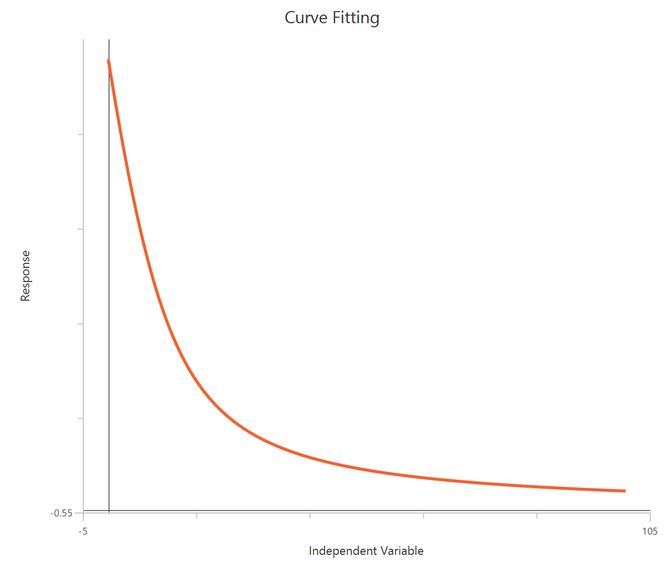
Input

The independent variable (X) must be the total inhibitor concentration on a linear scale and strictly positive (\(X>0\)). The dependent variable (Y) must be enzyme activity measured in consistent units (e.g., velocity in µM/min, absorbance change per minute, etc.). The following parameters must be provided and constrained to constant values based on independent experiments:

1. \(E_t\): Total concentration of enzyme catalytic sites (same concentration units as \(X\)).

2. \(S\): Substrate concentration used in the assay (same units as \(X\)).

3. \(K_m\): Michaelis–Menten constant determined in the absence of inhibitor (same units as \(X\)).

Parameters

1. \(V_{0}\): Enzyme velocity in the absence of inhibitor, expressed in the same units as \(Y\).

2. \(K_i\): Inhibition constant, expressed in the same units as \(X\). Smaller \(K_i\) values indicate tighter binding.

---

Exponential

One phase decay

The One phase decay model describes exponential decline processes in which the rate of decrease is proportional to the amount remaining. This behavior is characteristic of first-order kinetics and applies to many biological and chemical systems, including ligand dissociation, radioactive decay, and drug elimination. The model assumes a single homogeneous population decaying toward a stable plateau. The decay rate constant determines how rapidly the response approaches this asymptote.

Equation

\[ \begin{equation} Y = (Y_0 - \text{Plateau})\,e^{-KX} + \text{Plateau} \end{equation} \]

Visualization

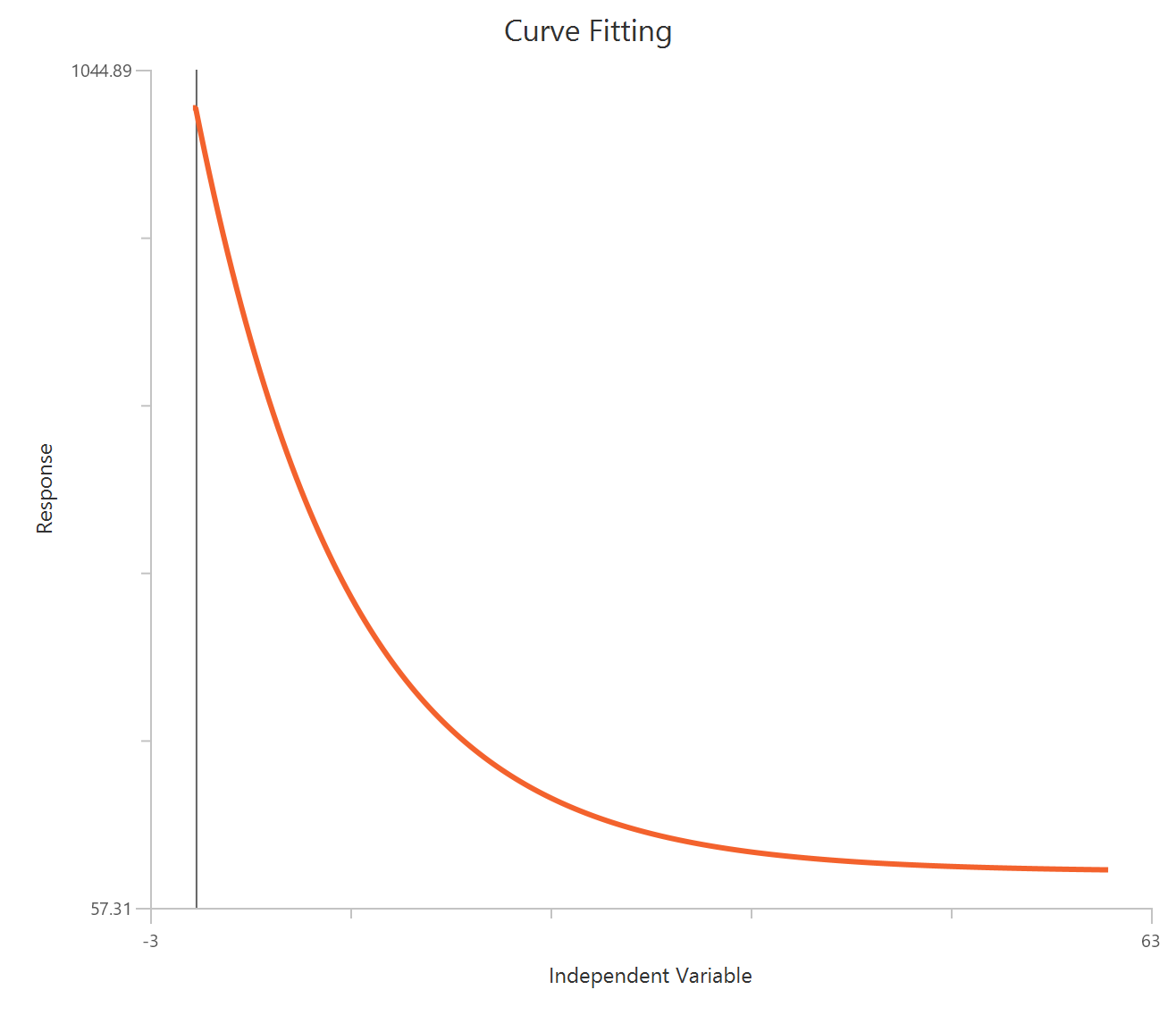
Input

The independent variable (X) must be on a linear scale and strictly positive (\(X>0\)). The model also requires a column containing the dependent variable (Y) response values (in any consistent units).

Parameters

1. \(Y_{0}\): The response value at time zero, expressed in the same units as \(Y\).

2. \(Plateau\): The response value as time approaches infinity. It represents the asymptotic minimum.

3. \(K\): The first-order rate constant (units are inverse time, e.g., \(min^{-1}\) or \(s^{-1}\)). \(K\) must be positive. Larger \(K\) values correspond to faster decay.

---

Two phase decay

The Two phase decay model describes processes in which the observed response is the sum of two independent first-order exponential decays: a fast component and a slow component. This situation arises when two kinetically distinct populations or mechanisms contribute to the signal (e.g., two binding states, two compartments, or heterogeneous molecular species). The total response declines toward a plateau as both components decay over time. The model assumes that each component follows first-order kinetics and that their contributions are additive.

Equation

\[ \begin{equation} \begin{aligned} \text{Span} &= Y_0 - \text{Plateau} \\ \text{Span}_{\text{Fast}} &= \text{Span}\cdot\frac{\text{PercentFast}}{100} \\ \text{Span}_{\text{Slow}} &= \text{Span}\cdot\frac{100 - \text{PercentFast}}{100} \end{aligned} \end{equation} \]

\[ \begin{equation} Y = \text{Plateau} + \text{Span}_{\text{Fast}}\,e^{-K_{\text{Fast}}X} + \text{Span}_{\text{Slow}}\,e^{-K_{\text{Slow}}X} \end{equation} \]

Visualization

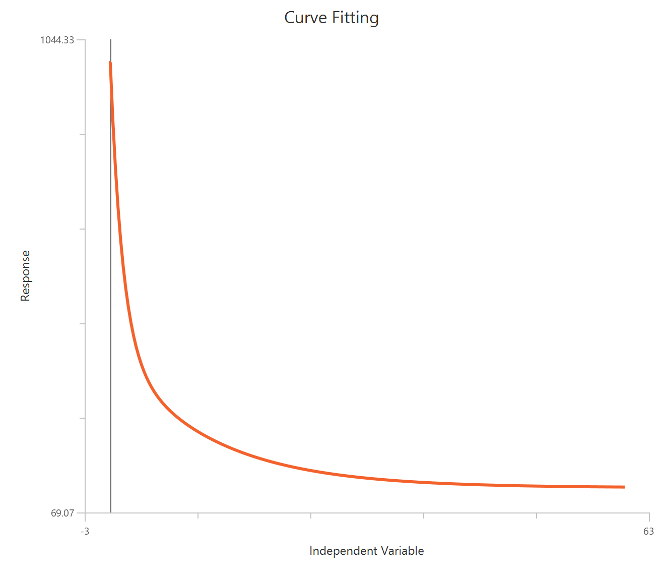
Input

The independent variable (X) must be on a linear scale and strictly positive (\(X>0\)). The model also requires a column containing the dependent variable (Y) response values (in any consistent units).

Parameters

1. \(Y_{0}\): The response value at time zero, expressed in the same units as \(Y\).

2. \(Plateau\): The response value as time approaches infinity. It represents the asymptotic minimum.

3. \(K_{Fast}\): Rate constant of the fast component (units: inverse time). Must be positive.

4. \(K_{Slow}\): Rate constant of the slow component (units: inverse time). Must be positive.

5. \(PercentFast\): Fraction (0–100%) of the total span attributed to the fast-decaying component.

---

Three phase decay

The Three phase decay model describes processes in which the observed response is the sum of three independent first-order exponential decays: fast, intermediate, and slow components. This model is appropriate when the signal arises from three kinetically distinct populations or mechanisms (e.g., multiple binding states or compartments). Each component decays exponentially and independently, and the total response is their sum plus a plateau value. Because this model contains several correlated parameters, reliable fitting requires dense time sampling and low experimental noise.

Equation

\[ \begin{equation} Y = \text{Plateau} + \text{Span}_{\text{Fast}}\,e^{-K_{\text{Fast}}X} + \text{Span}_{\text{Medium}}\,e^{-K_{\text{Medium}}X} + \text{Span}_{\text{Slow}}\,e^{-K_{\text{Slow}}X} \end{equation} \]

\[ \begin{equation} \begin{aligned} \text{Span} &= Y_0 - \text{Plateau} \\ \text{Span}_{\text{Fast}} &= \text{Span}\cdot\frac{\text{PercentFast}}{100} \\ \text{Span}_{\text{Slow}} &= \text{Span}\cdot\frac{\text{PercentSlow}}{100} \\ \text{Span}_{\text{Medium}} &= \text{Span} - \text{Span}_{\text{Fast}} - \text{Span}_{\text{Slow}} \end{aligned} \end{equation} \]

Visualization

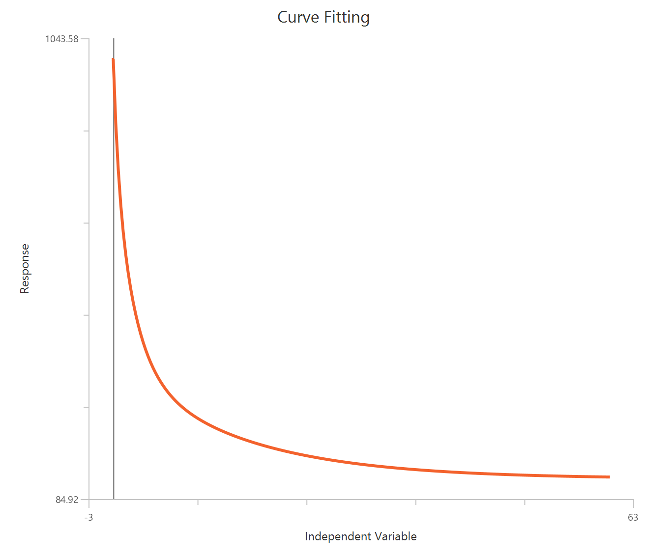
Input

The independent variable (X) must be on a linear scale and strictly positive (\(X>0\)). The model also requires a column containing the dependent variable (Y) response values (in any consistent units).

Parameters

1. \(Y_{0}\): The response value at time zero, expressed in the same units as \(Y\).

2. \(Plateau\): The response value as time approaches infinity. It represents the asymptotic minimum.

3. \(K_{Fast}\): Rate constant of the fast component (units: inverse time). Must be positive.

4. \(K_{Medium}\): Rate constant of the intermediate component (units: inverse time). Must be positive.

5. \(K_{Slow}\): Rate constant of the slow component (units: inverse time). Must be positive.

6. \(PercentFast\): Fraction (0–100%) of the total span attributed to the fast-decaying component.

7. \(PercentSlow\): Percentage (0–100%) of the total span attributed to the slow component.

---

Plateau followed by one phase decay

The Plateau followed by one phase decay model is a piecewise exponential-decay equation used when the response remains approximately constant for an initial period (baseline/plateau), and then begins to decay only after an intervention at a known (or fitted) start time \(X_0\). Before \(X_0\) the response is flat at \(Y_0\); after \(X_0\) it decays exponentially toward a final plateau. This is useful for experiments where decay is initiated by a washout, dilution, drug addition, temperature shift, or any trigger applied at a specific time.

Equation

\[ \begin{equation} Y = \begin{cases} Y_0, & X < X_0 \\ \text{Plateau} + (Y_0-\text{Plateau})\,e^{-K\,(X-X_0)}, & X \ge X_0 \end{cases} \end{equation} \]

\[ \begin{equation} \text{Span} = Y_0 - \text{Plateau} \end{equation} \]

Visualization

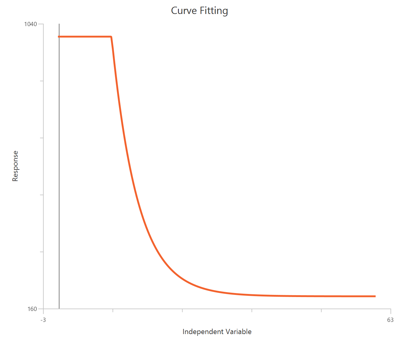
Input

The independent variable (X) must be on a linear scale and strictly positive (\(X>0\)). The model also requires a column containing the dependent variable (Y) response values (in any consistent units).

Parameters

1. \(X_0\): The time at which decay begins (same time units as \(X\)).

2. \(Y_{0}\): The baseline response level before decay begins (same units as \(Y\)). Conceptually, it is the plateau value for \(X<X_0\).

3. \(Plateau\): The response value as time approaches infinity. It represents the asymptotic minimum.

4. \(K\): The first-order decay rate constant (units: inverse time). \(K\) must be positive; larger \(K\) means faster decay after \(X_0\).

---

One phase association

The One phase association model describes pseudo–first-order association kinetics, where the response increases over time as binding/formation occurs and then approaches a steady-state plateau. Early in the experiment, many binding sites (or reactants) are available, so the response rises quickly; as sites become occupied, the rate of increase slows and the curve asymptotically approaches a maximum. This model is commonly used for simple association processes such as ligand–receptor binding, enzyme–substrate complex formation, or any system with a single dominant association phase.

Equation

\[ \begin{equation} Y = Y_0 + (\text{Plateau}-Y_0)\left(1-e^{-KX}\right) \end{equation} \]

\[ \begin{equation} \text{Span} = \text{Plateau} - Y_0 \end{equation} \]

Visualization

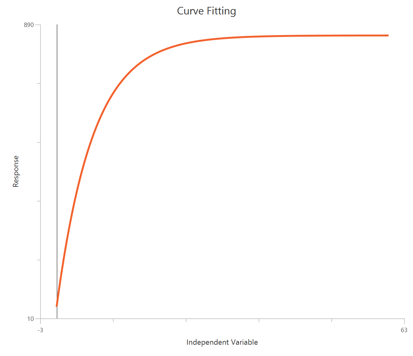
Input

The independent variable (X) must be on a linear scale and strictly positive (\(X>0\)). The model also requires a column containing the dependent variable (Y) response values (in any consistent units).

Parameters

1. \(Y_{0}\): The response at time zero (same units as \(Y\)).

2. \(Plateau\): The response at time zero (same units as \(Y\)). If background-subtracted data start at the origin, this can be fixed to 0.

3. \(K\): The association rate constant for the one-phase approach (units: inverse time). \(K\) must be positive; larger \(K\) means the curve reaches the plateau faster.

---

Two phase association

The Two phase association model describes a response that approaches a plateau through the sum of two independent exponential association processes: a fast component and a slow component. It is used when the measured response reflects two kinetically distinct populations or mechanisms (e.g., two receptor states, two binding sites, or parallel pathways). The curve rises rapidly at early times due to the fast component and then continues more slowly toward the same final plateau.

Equation

\[ \begin{equation} Y = Y_0 + \text{SpanFast}\left(1-e^{-K_{\text{Fast}}X}\right) + \text{SpanSlow}\left(1-e^{-K_{\text{Slow}}X}\right) \end{equation} \]

\[ \begin{equation} \text{SpanFast} = (\text{Plateau}-Y_0)\frac{\text{PercentFast}}{100} \end{equation} \]

\[ \begin{equation} \text{SpanSlow} = (\text{Plateau}-Y_0)\left(1-\frac{\text{PercentFast}}{100}\right) \end{equation} \]

Visualization

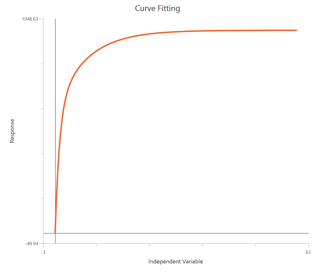
Input

The independent variable (X) must be on a linear scale and strictly positive (\(X>0\)). The model also requires a column containing the dependent variable (Y) response values (in any consistent units).

Parameters

1. \(Y_{0}\): The response at time zero (same units as \(Y\)).

2. \(Plateau\): The response at time zero (same units as \(Y\)). If background-subtracted data start at the origin, this can be fixed to 0.

3. \(K_{Fast}\): Rate constant of the fast association phase (units: inverse time). Larger values correspond to a more rapid initial rise.

4. \(K_{Slow}\): Rate constant of the slow association phase (units: inverse time).

5. \(PercentFast\): Percentage of the total span (\(Y_0\) to Plateau) attributable to the fast component (range 0–100).

---

Plateau followed by one phase association

The Plateau followed by one phase association model describes a system in which the response remains at a baseline level until a defined time point \(X_0\), after which a first-order association process begins. It is used when an experimental intervention (e.g., ligand addition, mixing, stimulus) initiates association at a known or fitted time rather than at \(X=0\). After \(X_0\), the response rises exponentially toward a plateau.

Equation

\[ \begin{equation} Y = \begin{cases} Y_0, & X < X_0 \\ Y_0 + (\text{Plateau}-Y_0)\left(1-e^{-K(X-X_0)}\right), & X \ge X_0 \end{cases} \end{equation} \]

Visualization

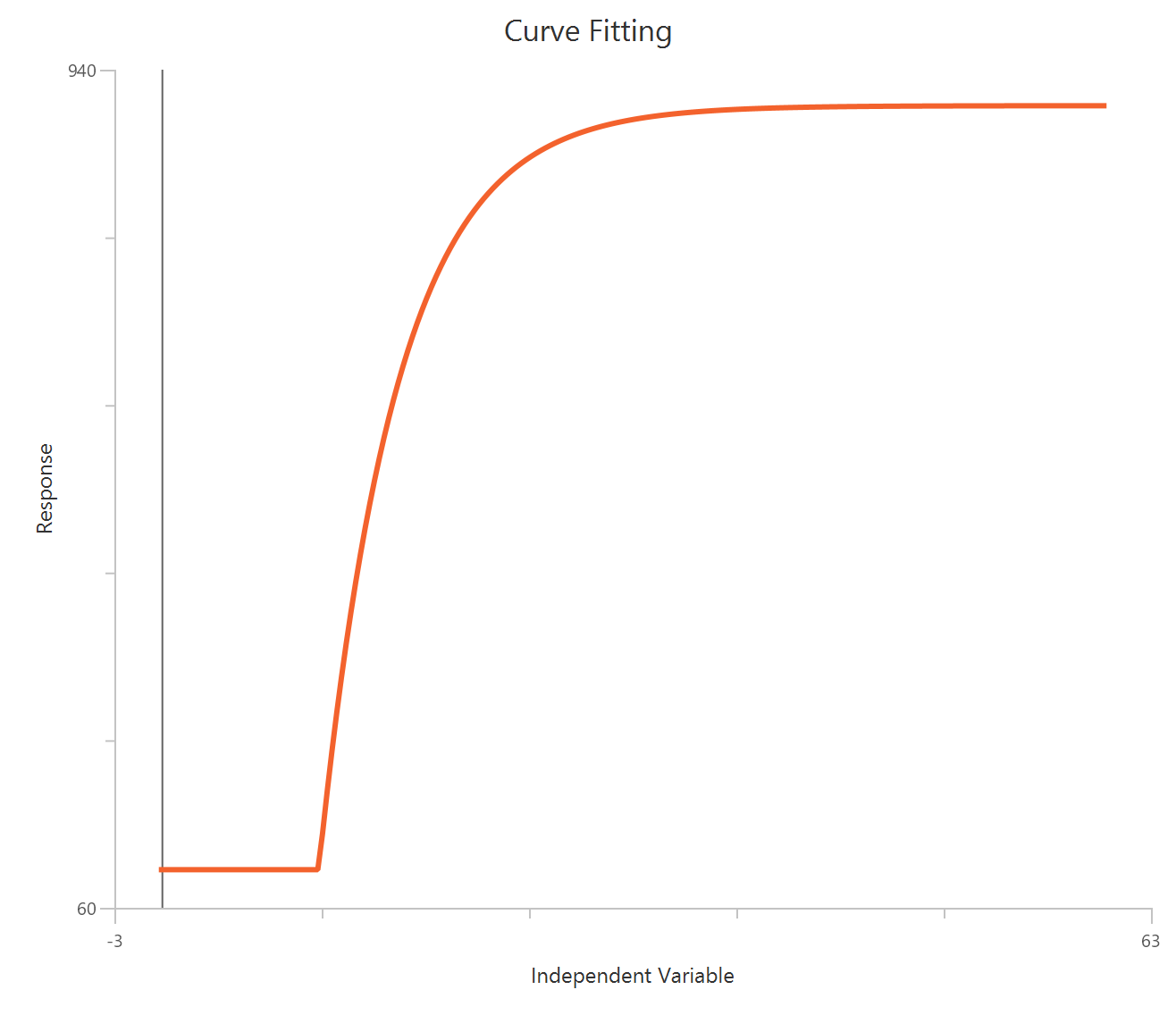
Input

The independent variable (X) must be on a linear scale and strictly positive (\(X>0\)). The model also requires a column containing the dependent variable (Y) response values (in any consistent units).

Parameters

1. \(X_0\): The time at which association begins (same time units as \(X\)).

2. \(Y_{0}\): The baseline response level before association begins (same units as \(Y\)). Conceptually, it is the plateau value for \(X<X_0\).

3. \(Plateau\): The response value as time approaches infinity. It represents the asymptotic minimum.

4. \(K\): Association rate constant (units: inverse time). Larger \(K\) produces a steeper rise.

---

Exponential Growth

The Exponential growth model describes processes that increase at a rate proportional to their current value. This produces growth with a constant doubling time. It is commonly used for population growth, cell proliferation, bacterial expansion, or compound accumulation under first-order kinetics.

Equation

\[ \begin{equation} Y = Y_0\, e^{KX} \end{equation} \]

Visualization

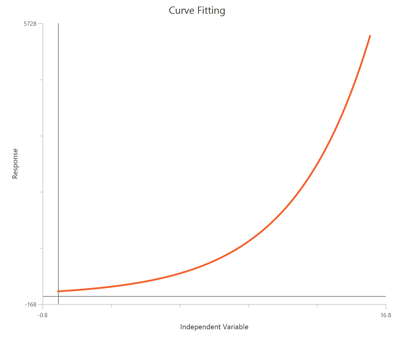
Input

The independent variable (X) must be on a linear scale and strictly positive (\(X>0\)). The model also requires a column containing the dependent variable (Y) response values (in any consistent units).

Parameters

1. \(Y_{0}\): The response at \(X=0\) (same units as \(Y\)).

2. \(K\): Growth rate constant (units: inverse time). Larger \(K\) produces faster growth.

---

Lines

Simple Line

The Simple line (nonlinear regression) model fits a linear relationship between an independent variable \(X\) and a dependent response \(Y\). Although the equation is linear in form, it is included here because it is fit using the nonlinear regression workflow, which can be useful when you want nonlinear-regression features (e.g., model comparison, weighting, or automatic outlier handling) while still fitting a straight line. The model assumes that changes in \(Y\) are proportional to changes in \(X\) across the measured range.

Equation

\[ \begin{equation} Y = Y_{\text{Intercept}} + \mathrm{Slope}\cdot X \end{equation} \]

Visualization

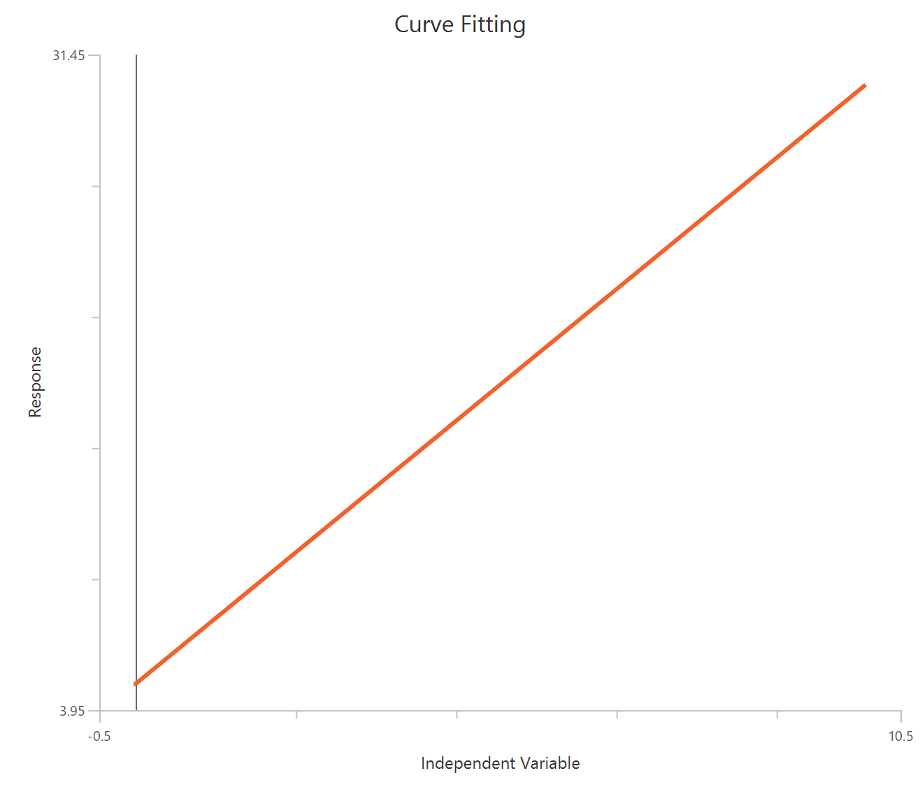
Input

The independent variable column \(X\) can be any real-valued numeric data (linear scale). The dependent variable column \(Y\) contains the response values in consistent units.

Parameters

1. \(Intercept\): The fitted value of \(X=0\) (the point where the line intersects the \(Y\)-axis). Units are the same as \(Y\).

2. \(Slope\): The slope of the fitted line, representing the change in \(Y\) per unit change in \(X\). Units are \(Y\)-units divided by \(X\)-units.

---

Simple Line through origin

The Simple Line through origin model fits a straight-line relationship between \(X\) and \(Y\) while forcing the intercept to be exactly zero. This is appropriate when theory or experimental design requires that \(Y=0\) when \(X=0\) (i.e., the relationship must pass through the origin). Because the intercept is fixed, the only fitted parameter is the slope, which represents the proportionality between \(Y\) and \(X\).

Equation

\[ \begin{equation} Y = \mathrm{Slope}\cdot X \end{equation} \]

Visualization

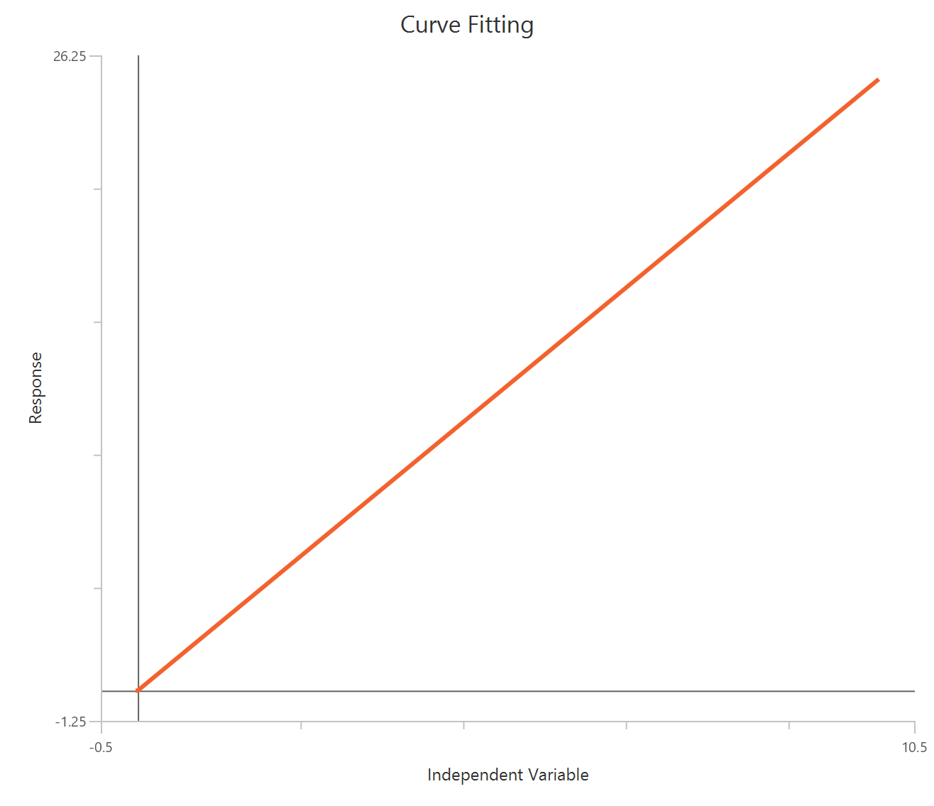
Input

The independent variable column \(X\) can be any real-valued numeric data (linear scale). The dependent variable column \(Y\) contains the response values in consistent units.

Parameters

1. \(Slope\): The slope of the fitted line, representing the change in \(Y\) per unit change in \(X\). Units are \(Y\)-units divided by \(X\)-units.

---

Simple Line through (X0,Y0)

The Simple line through \((X_0,Y_0)\) model fits a straight line while forcing it to pass through a specified point \((X_0,Y_0)\). This is useful when you know one exact calibration/reference point that the fitted relationship must satisfy (e.g., a baseline measurement, a normalization anchor, or a physical constraint). The model estimates a single parameter (Slope), while the intercept is implied by the requirement that the line passes through \((X_0,Y_0)\).

Equation

\[ \begin{equation} Y = Y_0 + \mathrm{Slope}\,(X - X_0) \end{equation} \]

Visualization

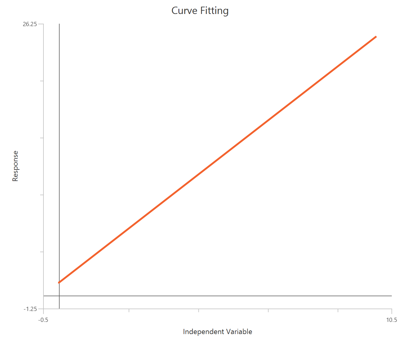
Input

The independent variable column \(X\) can be any real-valued numeric data (linear scale). The dependent variable column \(Y\) contains the response values in consistent units.

Parameters

1. \(Slope\): The slope of the fitted line, representing the change in \(Y\) per unit change in \(X\). Units are \(Y\)-units divided by \(X\)-units.

---

Segmental linear regression (2 segments)

Segmental linear regression (also called piecewise or segmented regression) fits two straight-line segments with a single breakpoint at \(X_0\). One line is used for \(X < X_0\) and a second line is used for \(X≥X_0\), with continuity enforced so the two segments meet exactly at \(X_0\). This is useful when the relationship changes slope abruptly at a known or unknown transition point (e.g., an intervention time, a threshold effect, or a regime change).

Equation

\[ \begin{equation} \begin{aligned} Y_1 &= \mathrm{Intercept}_1 + \mathrm{Slope}_1\,X \\ Y_{\text{at}X_0} &= \mathrm{Intercept}_1 + \mathrm{Slope}_1\,X_0 \\ Y_2 &= Y_{\text{at}X_0} + \mathrm{Slope}_2\,(X - X_0) \\ Y &= \mathrm{IF}(X<X_0,\; Y_1,\; Y_2) \end{aligned} \end{equation} \]

Visualization

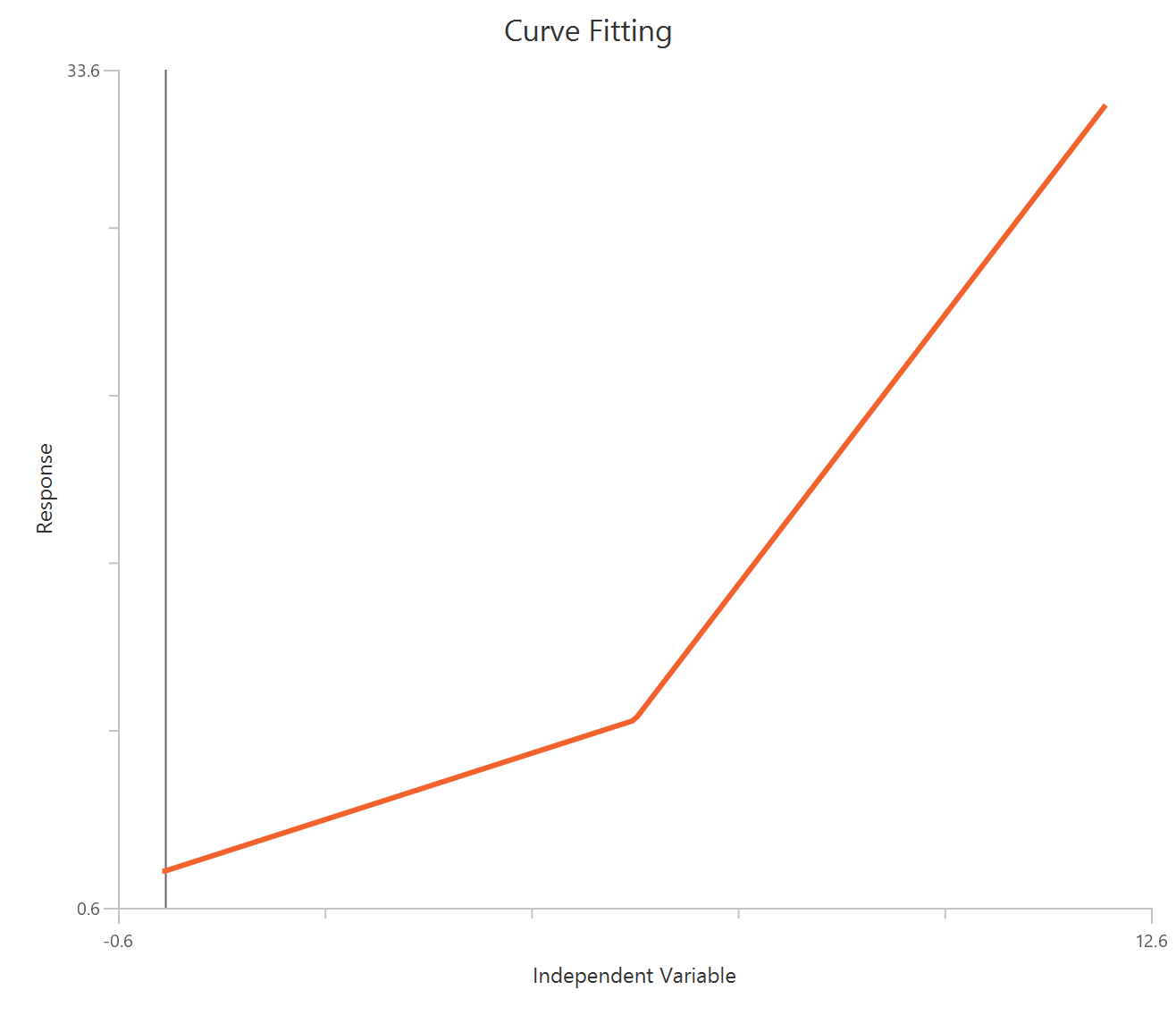
Input

The independent variable column \(X\) can be any real-valued numeric data (linear scale). The dependent variable column \(Y\) contains the response values in consistent units. The model requires the sepcification of one extra parameter:

1. \(X_0\): The breakpoint (the \(X\) value where the slope changes). This is the X value where the model switches from the first line to the second, with continuity enforced at \(X_0\).

Parameters

1. \(Intercept\): The \(Y\)-intercept of the first segment (units: \(Y\)). It is the predicted \(Y\) value when \(X=0\) according to the first line.

2. \(Slope_1\): The slope of the first segment (units: \(Y\) per \(X\)). It describes how \(Y\) changes with \(X\) for \(X<X_0\).

3. \(Slope_2\): The slope of the second segment (units: \(Y\) per \(X\)). It describes how \(Y\) changes with \(X\) for \(X \geq X_0\).

---

Segmental linear regression (3 segments)

This three-segment (piecewise) linear regression fits three straight-line segments separated by two breakpoints, \(X_0\) and \(X_1\). The model uses one line for \(X < X_0\), a second line for \(X_0 \leq X < X_1\), and a third line for \(X \geq X_1\). Continuity is enforced so the segments meet exactly at both breakpoints.

Equation

\[ \begin{equation} \begin{aligned} Y_1 &= \mathrm{Intercept}_1 + \mathrm{Slope}_1\,X \\ Y_{\text{at}X_0} &= \mathrm{Intercept}_1 + \mathrm{Slope}_1\,X_0 \\ Y_2 &= Y_{\text{at}X_0} + \mathrm{Slope}_2\,(X - X_0) \\ Y_{\text{at}X_1} &= Y_{\text{at}X_0} + \mathrm{Slope}_2\,(X_1 - X_0) \\ Y_3 &= Y_{\text{at}X_1} + \mathrm{Slope}_3\,(X - X_1) \\ Y &= \mathrm{IF}(X<X_0,\; Y_1,\; \mathrm{IF}(X<X_1,\; Y_2,\; Y_3)) \end{aligned} \end{equation} \]

Visualization

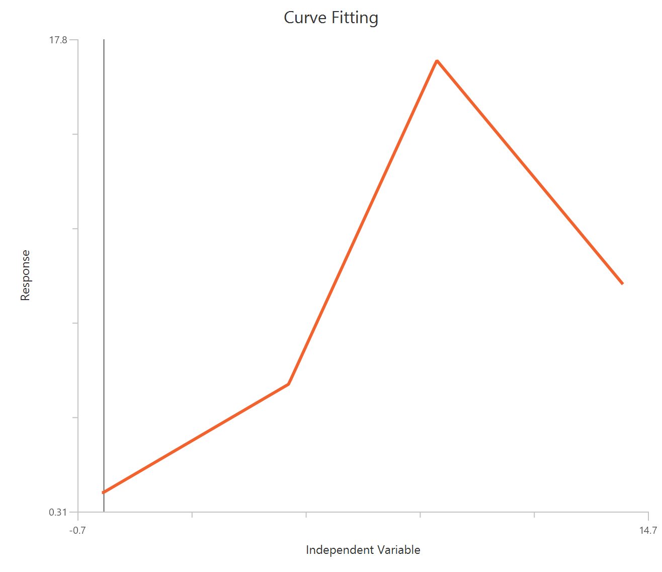
Input

The independent variable column \(X\) can be any real-valued numeric data (linear scale). The dependent variable column \(Y\) contains the response values in consistent units. The model requires the sepcification of two extra parameters:

1. \(X_0\): The first breakpoint provided by the user (units: \(X\)). The model switches from segment 1 to segment 2 at \(X_0\).
2. \(X_1\): The second breakpoint provided by the user (units: \(X\)). The model switches from segment 2 to segment 3 at \(X_1\).

Parameters

1. \(Intercept\): The \(Y\)-intercept of the first segment (units: \(Y\)). It is the predicted \(Y\) value when \(X=0\) according to the first line.

2. \(Slope_1\): The slope of the first segment (units: \(Y\) per \(X\)). It describes how \(Y\) changes with \(X\) for \(X<X_0\).

3. \(Slope_2\): The slope of the second segment (units: \(Y\) per \(X\)). It describes how \(Y\) changes with \(X\) for \(X_0 \leq X < X_1\).

4. \(Slope_3\): The slope of the third segment (units: \(Y\) per \(X\)). It describes how \(Y\) changes with \(X\) for \(X \geq X_1\).

---

Hinge function

The hinge function fits two approximately linear segments joined by a smooth transition rather than a sharp corner. For values of \(X\) far below the breakpoint \(X_0\), the curve behaves like a straight line with slope \(Slope_1\). For values far above \(X_0\), it approaches a second straight line with slope Slope_2. The transition between these two slopes is controlled by the parameter \(Δ\), which determines how gradual the bend is. There is also an option to constrain \(Δ\) using the Hinge function (fixed \(Δ\) equation.)

When \(Δ→0\), the model approaches ordinary segmented (piecewise) linear regression with two intersecting straight lines. Larger \(Δ\) values produce a smoother, more gradual change in slope.

Equation

\[ \begin{equation} Y = \mathrm{Intercept} + \mathrm{Slope}_1 (X - X_0) + (\mathrm{Slope}_2 - \mathrm{Slope}_1)\,\Delta \,\ln\!\left(1 + \exp\!\left(\frac{X - X_0}{\Delta}\right)\right) \end{equation} \]

Visualization

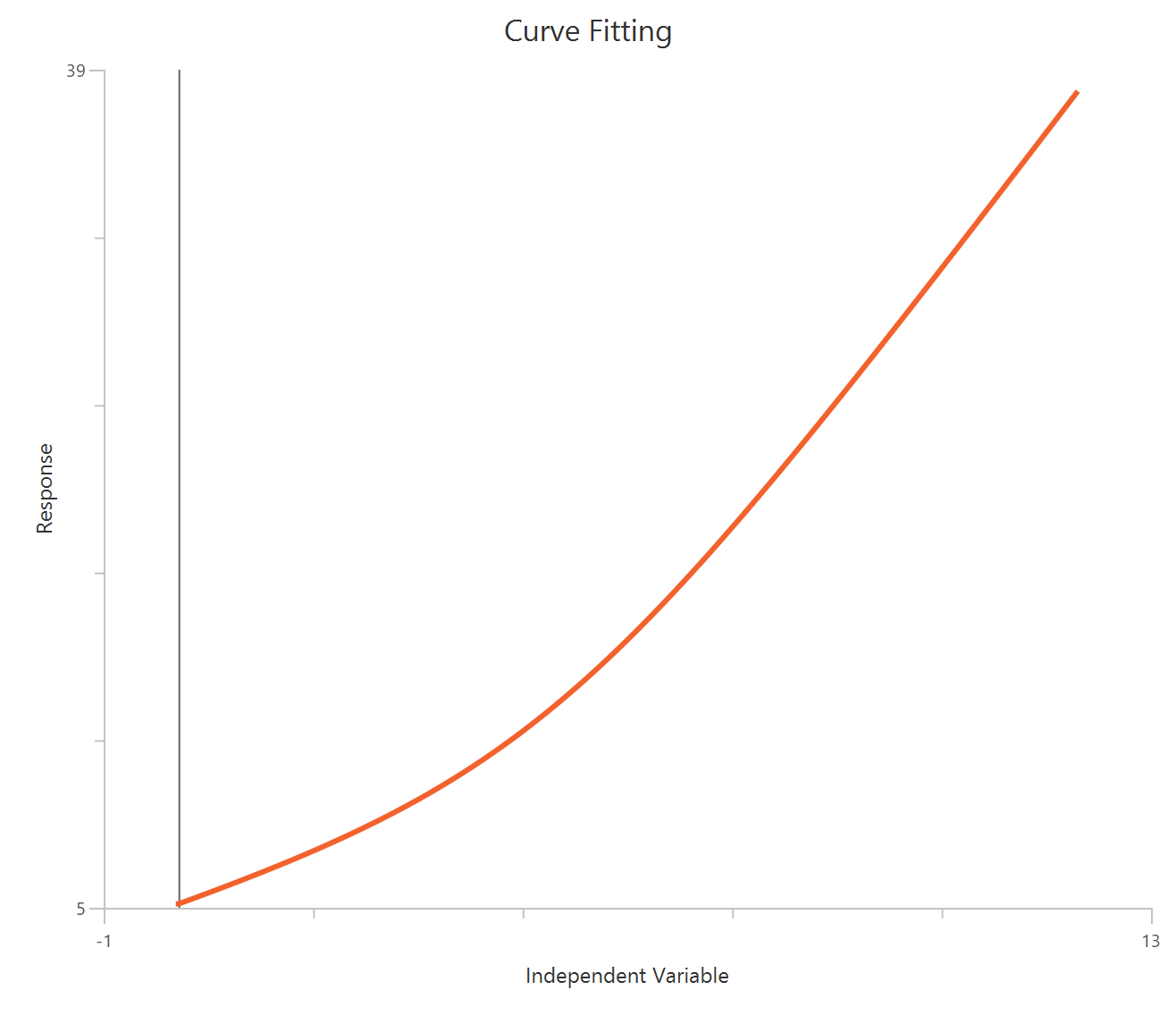
Input

The independent variable column \(X\) can be any real-valued numeric data (linear scale). The dependent variable column \(Y\) contains the response values in consistent units. The model requires the sepcification of two extra parameters:

1. \(X_0\): The breakpoint provided by the user (units: \(X\)). The model switches from segment 1 to segment 2 at \(X_0\).

Parameters

1. \(Intercept\): The \(Y\)-intercept of the first segment (units: \(Y\)). It is the predicted \(Y\) value when \(X=0\) according to the first line.

2. \(Slope_1\): The slope of the first segment (units: \(Y\) per \(X\)). It describes how \(Y\) changes with \(X\) for \(X<X_0\).

3. \(Slope_2\): The slope of the second segment (units: \(Y\) per \(X\)). It describes how \(Y\) changes with \(X\) for \(X_0 \leq X\).

4. \(\Delta\): The smoothness parameter (units of \(X\)). It controls how sharp or gradual the bend is. It must be strictly positive.

   1. As \(Δ→0\), the model approaches two intersecting straight lines.
   2. Larger \(Δ\) values produce a more gradual transition.

---

Polynomial

Polynomial Models (order 1-6)

Polynomial models provide a flexible, empirical way to describe the relationship between an independent variable \(X\) and a response \(Y\) by expressing \(Y\) as a finite sum of powers of \(X\). Increasing the polynomial order adds additional curvature and can improve fit, but higher-order polynomials may also introduce unnecessary “wiggles” and overfit noise. Because polynomial models are typically used for interpolation/smoothing rather than to represent an underlying mechanistic process, the coefficients are often not directly interpretable.

Equation

\[ \begin{equation} Y = B_0 + B_1X + B_2X^2 + \cdots + B_nX^n \end{equation} \]

\[ \begin{equation} \begin{aligned} \text{First order:}\quad & Y = B_0 + B_1X \\ \text{Second order:}\quad & Y = B_0 + B_1X + B_2X^2 \\ \text{Third order:}\quad & Y = B_0 + B_1X + B_2X^2 + B_3X^3 \\ \text{Fourth order:}\quad & Y = B_0 + B_1X + B_2X^2 + B_3X^3 + B_4X^4 \\ \text{Fifth order:}\quad & Y = B_0 + B_1X + B_2X^2 + B_3X^3 + B_4X^4 + B_5X^5 \\ \text{Sixth order:}\quad & Y = B_0 + B_1X + B_2X^2 + B_3X^3 + B_4X^4 + B_5X^5 + B_6X^6 \end{aligned} \end{equation} \]

Visualization

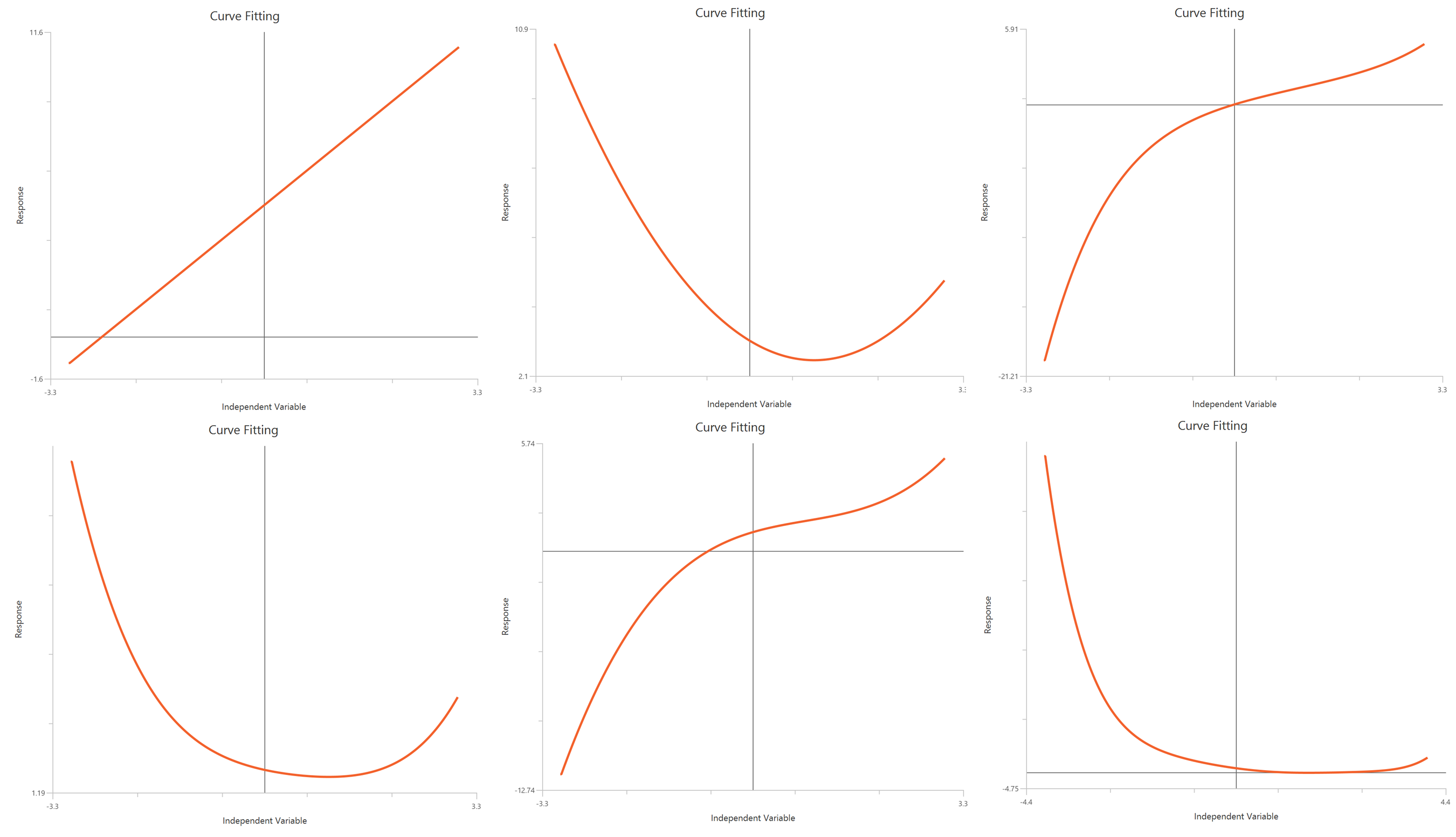
Input

The independent variable (X) must be on a linear scale. The model also requires a column containing the dependent variable (Y) response values (in any consistent units).

Parameters

1. \(B_{0}\): Intercept term (value of the polynomial at \(X=0\)).

2. \(B_1,B_2,...,B_n\): Polynomial coefficients for the linear, quadratic, …, n-th order terms.

---

Centered Polynomial Models (order 1-6)

Centered polynomial models are algebraically equivalent to ordinary polynomial models, but instead of using \(X\) directly, they use a centered variable defined as the deviation from the mean of \(X\). Centering improves numerical stability, reduces parameter covariance, and yields tighter standard errors and confidence intervals — especially for higher-order polynomials or when \(X\) values are large.

In centered models, the mean of the independent variable is subtracted before fitting:

\[ \begin{equation} X_{C} = X - X_{mean} \end{equation} \]

where \(X_{mean}\) is the mean of all \(X\) values used in the fit. This quantity is treated as a constant (data-set constant), not as a fitted parameter.

Equation

\[ \begin{aligned} \textbf{First order:}\quad & Y = B_0 + B_1(X - X_{\text{mean}}) \\[6pt] \\ \textbf{Second order:}\quad & Y = B_0 + B_1(X - X_{\text{mean}}) + B_2(X - X_{\text{mean}})^2 \\[6pt] \\ \textbf{Third order:}\quad & Y = B_0 + B_1(X - X_{\text{mean}}) + B_2(X - X_{\text{mean}})^2 \\ & \qquad + B_3(X - X_{\text{mean}})^3 \\[6pt] \\ \textbf{Fourth order:}\quad & Y = B_0 + B_1(X - X_{\text{mean}}) + B_2(X - X_{\text{mean}})^2 \\ & \qquad + B_3(X - X_{\text{mean}})^3 + B_4(X - X_{\text{mean}})^4 \\[6pt] \\ \textbf{Fifth order:}\quad & Y = B_0 + B_1(X - X_{\text{mean}}) + B_2(X - X_{\text{mean}})^2 \\ & \qquad + B_3(X - X_{\text{mean}})^3 + B_4(X - X_{\text{mean}})^4 \\ & \qquad + B_5(X - X_{\text{mean}})^5 \\[6pt] \\ \textbf{Sixth order:}\quad & Y = B_0 + B_1(X - X_{\text{mean}}) + B_2(X - X_{\text{mean}})^2 \\ & \qquad + B_3(X - X_{\text{mean}})^3 + B_4(X - X_{\text{mean}})^4 \\ & \qquad + B_5(X - X_{\text{mean}})^5 + B_6(X - X_{\text{mean}})^6 \end{aligned} \]

Visualization

Input

The independent variable (X) must be on a linear scale. The model also requires a column containing the dependent variable (Y) response values (in any consistent units). The model requires the specification of one extra parameter:

1. \(X_{mean}\): The mean of the X values.

Parameters

1. \(B_{0}\): Intercept term (value of the polynomial at \(X=X_{mean}\)).

2. \(B_1,B_2,...,B_n\): Polynomial coefficients for the linear, quadratic, …, n-th order terms.

---

Gaussian

Gaussian Distribution

The Gaussian (normal) distribution describes symmetric, bell-shaped frequency distributions that arise when variability is driven by many independent, additive factors. In histogram fitting, the X values represent bin centers and the Y values represent frequencies (counts).

Equation

\[ \begin{equation} Y = \mathrm{Amplitude} \cdot \exp\!\left(-\frac{1}{2}\left(\frac{X - \mathrm{Mean}}{\mathrm{SD}}\right)^2\right) \end{equation} \]

Visualization

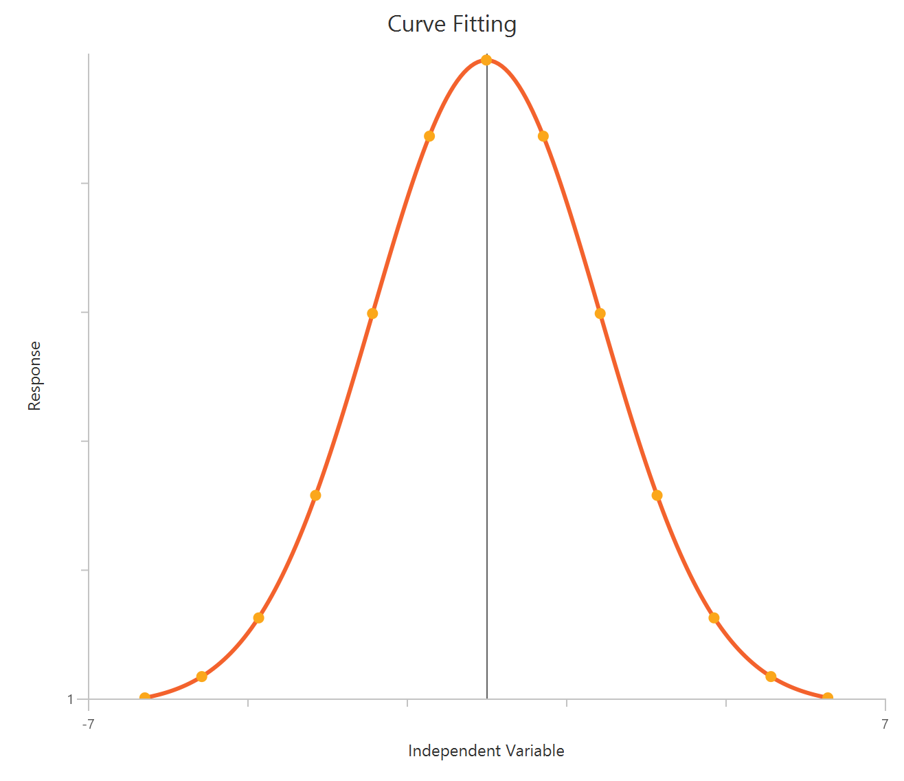
Input

The independent variable (X) must be Bin centers of the frequency distribution (linear scale). The model also requires a column containing the dependent variable (Y) as the observed frequency (number of observations) in each bin.

Parameters

1. \(Amplitude\): The peak height of the distribution (maximum \(Y\) value). Units: same as \(Y\).

2. \(Mean\): The center of the distribution (location of the peak). Units: same as \(X\).

3. \(SD\): The standard deviation, describing the spread (width) of the distribution. Units: same as \(X\).

---

Sum of two Gaussian Distributions

The Sum of two Gaussian distributions model is used when a frequency distribution (histogram-style XY table) appears to be a mixture of two underlying normal populations. The observed counts are modeled as the sum of two bell-shaped Gaussian components, each with its own center and spread.

Equation

\[ \begin{aligned} Y &= \mathrm{One} + \mathrm{Two} \\ \mathrm{One} &= \mathrm{Amplitude1}\cdot \exp\!\left(-0.5\left(\frac{X-\mathrm{Mean1}}{\mathrm{SD1}}\right)^2\right) \\ \mathrm{Two} &= \mathrm{Amplitude2}\cdot \exp\!\left(-0.5\left(\frac{X-\mathrm{Mean2}}{\mathrm{SD2}}\right)^2\right) \end{aligned} \]

Visualization

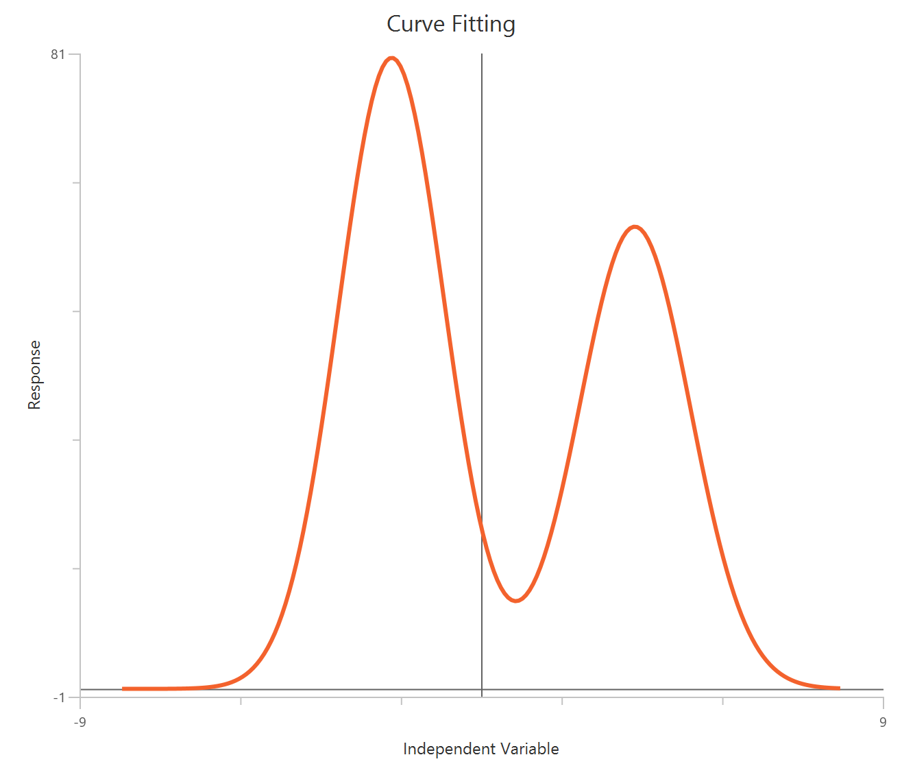
Input

The independent variable (X) must be Bin centers of the frequency distribution (linear scale). The model also requires a column containing the dependent variable (Y) as the observed frequency (number of observations) in each bin.

Parameters

1. \(Amplitude_1\): The peak height of the first distribution (maximum \(Y\) value). Units: same as \(Y\).

2. \(Mean_1\): The center of the first distribution (location of the peak). Units: same as \(X\).

3. \(SD_1\): The standard deviation, describing the spread (width) of the first distribution. Units: same as \(X\).

4. \(Amplitude_2\): The peak height of the second distribution (maximum \(Y\) value). Units: same as \(Y\).

5. \(Mean_2\): The center of the second distribution (location of the peak). Units: same as \(X\).

6. \(SD_2\): The standard deviation, describing the spread (width) of the second distribution. Units: same as \(X\).

---

Lognormal Distribution

The Lognormal distribution model is used to fit frequency distributions when the logarithm of the variable is normally distributed. Such data arise when variability results from the product (rather than the sum) of many independent, positive factors. On a linear X-axis the distribution is right-skewed; on a logarithmic X-axis it appears Gaussian.

Equation

\[ Y = \frac{A}{X}\,\exp\!\left(-\frac{1}{2}\left(\frac{\ln(X/\mathrm{GeoMean})}{\ln(\mathrm{GeoSD})}\right)^2\right) \]

Visualization

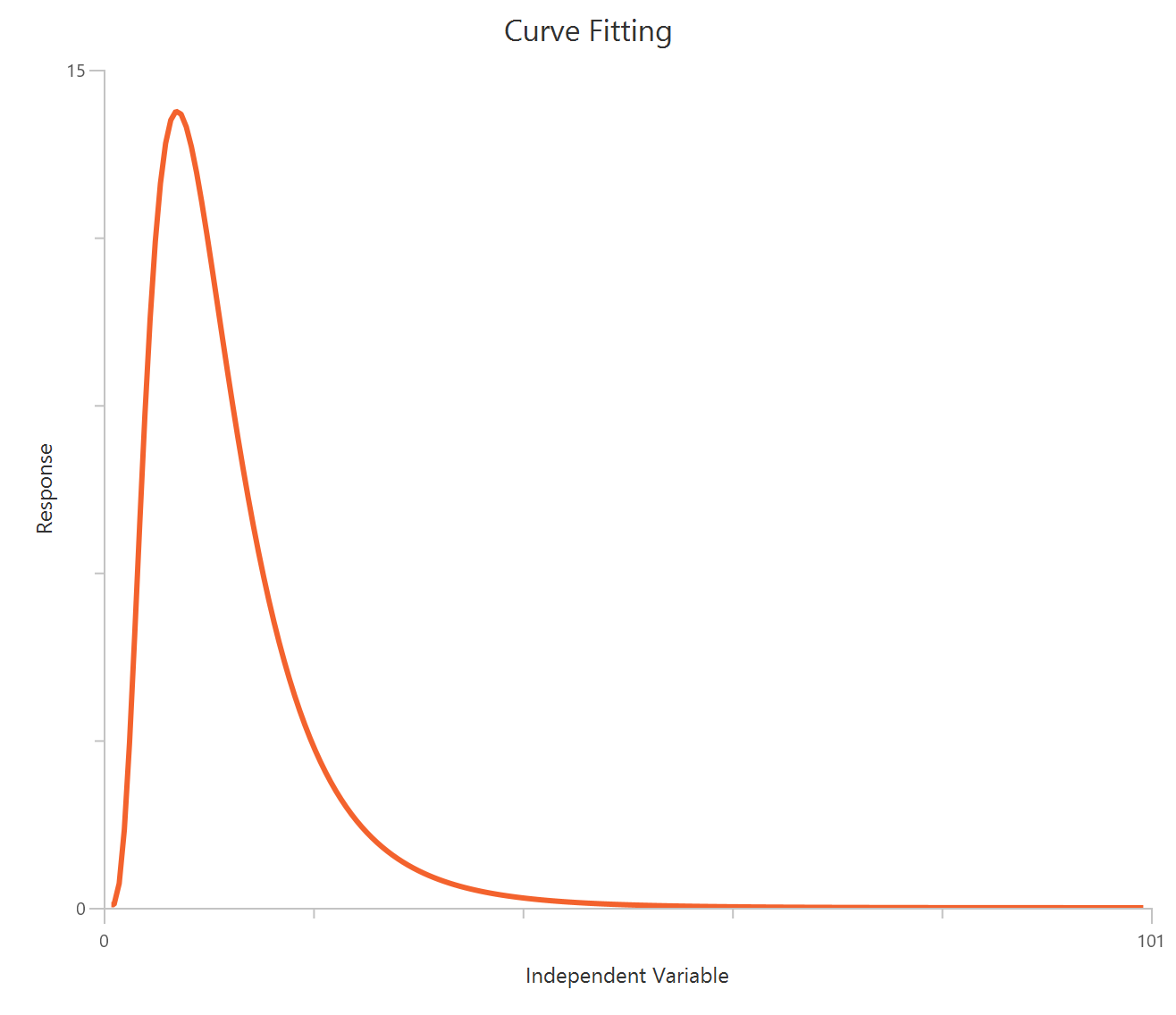
Input

The independent variable (X) must be Bin centers of the frequency distribution (positive values only).Zero or negative X values are not used in the calculations (they are ignored/excluded). The model also requires a column containing the dependent variable (Y) as the observed frequency (number of observations) in each bin.

Parameters

1. \(A\): A scaling constant related to the total area under the curve.

2. \(GeoMean\): The geometric mean of the distribution. Units: same as \(X\).

3. \(GeoSD\): The geometric standard deviation factor (dimensionless). It determines the spread of the distribution on a logarithmic scale.

---

Cumulative Gaussian distribution

The Cumulative Gaussian distribution model fits cumulative frequency data derived from an underlying Gaussian (normal) distribution. Instead of plotting the frequency within bins, the cumulative distribution plots the number (or fraction or percentage) of observations less than or equal to each value of \(X\).

If the underlying data follow a Gaussian distribution, the cumulative plot has a sigmoidal (S-shaped) form.

Equation

There are three forms of the model, depending on whether \(Y\) values represent percentages, fractions, or counts.

1. When \(Y\) is in percentages (0–100) [ Y = 100 \cdot \Phi(z) ]:

\[ z = \frac{X - \mathrm{Mean}}{\mathrm{SD}} \]

1. When \(Y\) is in fractions (0–1) \(Y = \Phi(z)\):

\[ z = \frac{X - \mathrm{Mean}}{\mathrm{SD}} \]

1. When \(Y\) is counts (number of observations) \(Y = N \cdot \Phi(z)\):

\[ z = \frac{X - \mathrm{Mean}}{\mathrm{SD}} \]

Where: \(\Phi(z) = \frac{1}{\sqrt{2\pi}} \int_{-\infty}^{z} e^{-t^2/2} dt\) is the cumulative distribution function (CDF) of the standard normal distribution.

Visualization

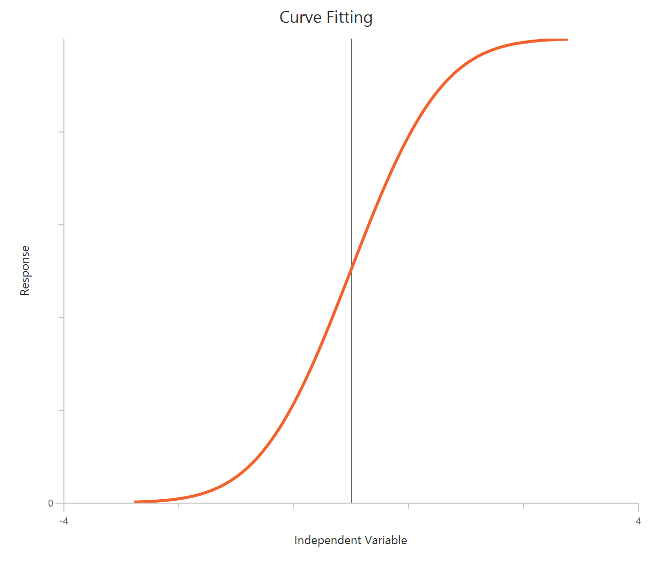
Input

The independent variable (X) must be Bin centers of the frequency distribution. The model also requires a column containing the dependent variable (Y) as the cumulative percent/fraction or count of observaitions less than or equal to each \(X\) value. If \(Y\) contains counts, constrain \(N\) to a constant equal to the total number of observations.

Parameters

1. \(Mean\): The mean of the underlying Gaussian distribution (same units as \(X\)).

2. \(SD\): The standard deviation of the underlying Gaussian distribution (same units as \(X\)).

---

Lorentzian Distribution

The Lorentzian (Cauchy) distribution is a bell-shaped frequency distribution with much heavier tails than a Gaussian distribution. It is often used when extreme values/outliers occur more frequently than a normal model would predict. In curve fitting, it is commonly applied to histogram-style frequency data, where \(X\) represents bin centers and \(Y\) is the number of observations in each bin.

Equation

\[ \begin{equation} Y = \frac{\mathrm{Amplitude}}{1 + \left(\frac{X-\mathrm{Center}}{\mathrm{Width}}\right)^2} \end{equation} \]

Visualization

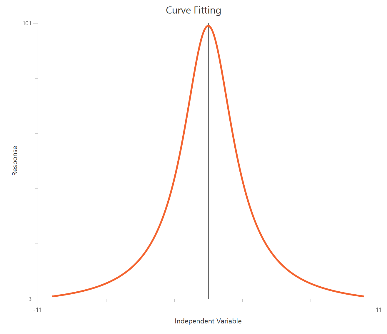
Input

The independent variable (X) must be Bin centers of the frequency distribution (linear scale). The model also requires a column containing the dependent variable (Y) as the observed frequency (number of observations) in each bin.

Parameters

1. \(A\): Peak height of the distribution (in \(Y\) units). This is the value of \(Y\) when \(X=Center\).

2. \(Center\): Location of the peak (same units as \(X\)). It is the \(X\) value at which the distribution is maximal.

3. \(Width\): A width (scale) parameter (same units as \(X\)). Larger \(Width\) produces a broader peak with heavier spread.

---

Sum of two Lorentzian Distributions

This model describes data arising from the sum of two Lorentzian (Cauchy) components, each with its own center and width. It is commonly used when a frequency distribution exhibits two overlapping heavy-tailed peaks.

Equation

\[ \begin{equation} Y = \frac{\mathrm{Amplitude1}}{1 + \left(\frac{X-\mathrm{Center1}}{\mathrm{Width1}}\right)^2} + \frac{\mathrm{Amplitude2}}{1 + \left(\frac{X-\mathrm{Center2}}{\mathrm{Width2}}\right)^2} \end{equation} \]

Visualization

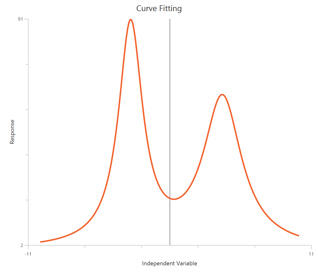
Input

The independent variable (X) must be Bin centers of the frequency distribution (linear scale). The model also requires a column containing the dependent variable (Y) as the observed frequency (number of observations) in each bin.

Parameters

1. \(A_1\): Peak height of the first distribution (in \(Y\) units). This is the value of \(Y\) when \(X=Center\).

2. \(Center_1\): Location of the peak of the first distribution (same units as \(X\)). It is the \(X\) value at which the first distribution is maximal.

3. \(Width_1\): A width (scale) parameter for the first distribution (same units as \(X\)). Larger \(Width\) produces a broader peak with heavier spread.

4. \(A_2\): Peak height of the second distribution (in \(Y\) units). This is the value of \(Y\) when \(X=Center\).

5. \(Center_2\): Location of the peak of the second distribution (same units as \(X\)). It is the \(X\) value at which the second distribution is maximal.

6. \(Width_2\): A width (scale) parameter for the second distribution (same units as \(X\)). Larger \(Width\) produces a broader peak with heavier spread.

---

Sine Waves

Standard Sine wave

The Standard sine wave model describes a periodic oscillatory process with constant amplitude and wavelength. The response varies sinusoidally with respect to the independent variable and is defined by three parameters: amplitude (peak magnitude), wavelength (period of oscillation), and phase shift (horizontal displacement of the wave).

Equation

\[ \begin{equation} Y = \mathrm{Amplitude}\,\sin\!\left(\frac{2\pi X}{\mathrm{Wavelength}} + \mathrm{PhaseShift}\right) \end{equation} \]

Visualization

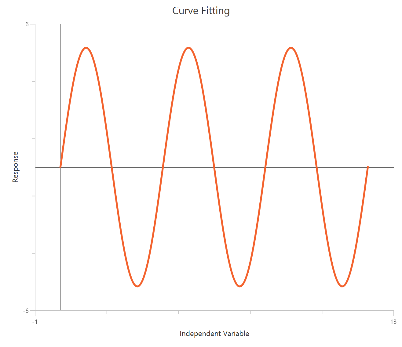
Input

The independent variable (X) is typically time, angle, or spatial position and may take positive or negative values. The dependent variable (Y) represents the oscillatory response and can be in any consistent units. X must be on a linear scale.

Parameters

1. \(Amplitude\): The peak magnitude of the oscillation (in Y units). The wave oscillates between \(+Amplitude$ and\)−Amplitude$$.

2. \(Wavelength\): The length of one complete cycle (same units as X). It determines how frequently the oscillation repeats.

3. \(PhaseShift\): The phase offset (in radians). It shifts the waveform horizontally along the X-axis.

   1. If \(PhaseShift=0\), then \(Y=0\) at \(X=0\).
   2. If \(PhaseShift=\pi/2\), the function is at its maximum at at \(X=0\).

---

Damped Sine wave

The Damped sine wave model describes oscillatory behavior whose amplitude decreases exponentially over time (or over the X variable). It is appropriate for systems where repeated cycles persist but energy is lost (damping), so peaks shrink as X increases. The oscillation itself is governed by a sine function (with wavelength and phase shift), while the damping envelope is controlled by an exponential decay term with decay constant \(K\).

Equation

\begin{equation} Y = Amplitude \cdot e^{-KX}\cdot \sin\left(\frac{2\pi X}{Wavelength}\right) + PhaseShift \end{equation}

Visualization

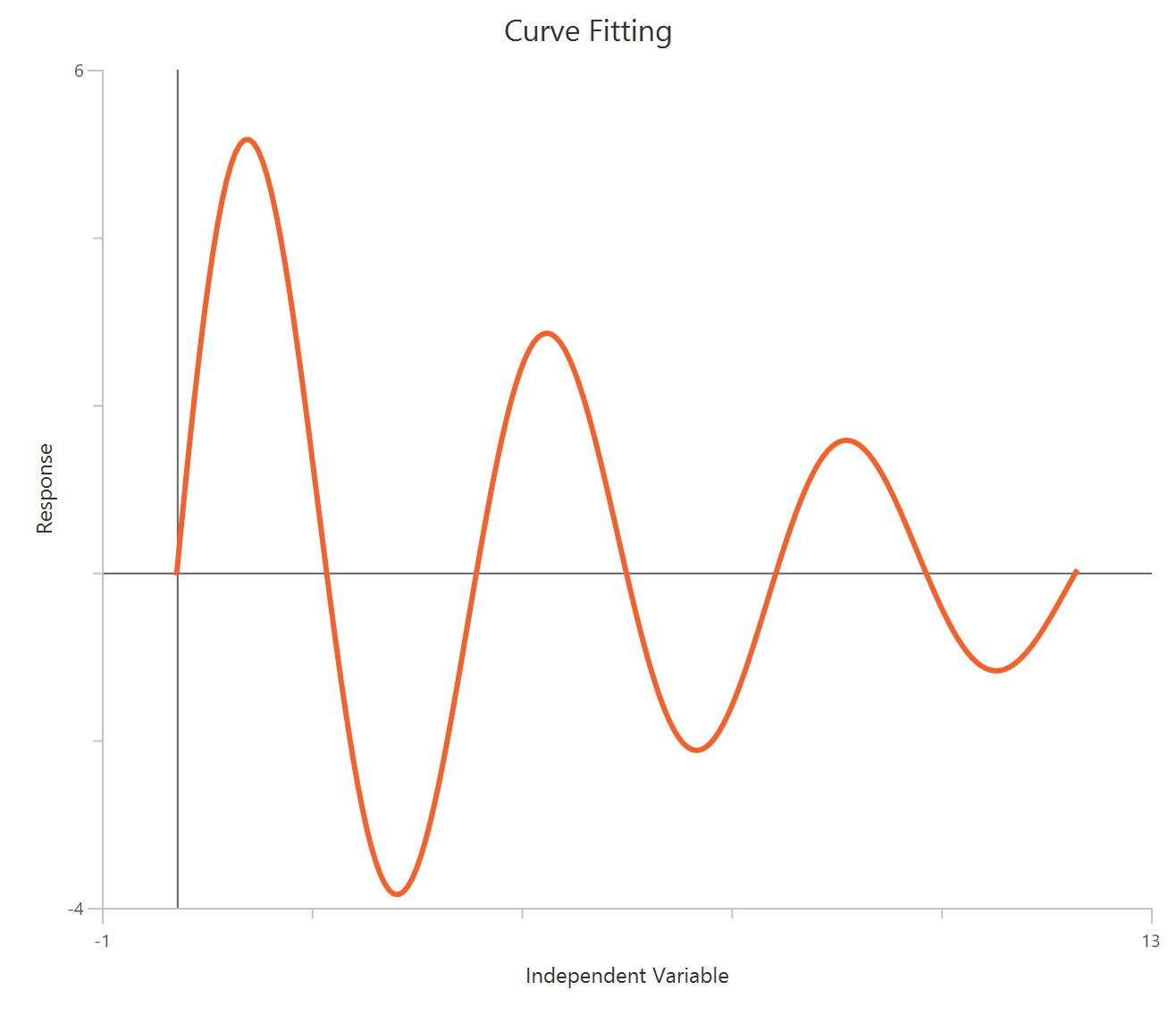
Input

The independent variable (X) is typically time (or any linear-scale variable along which damping occurs) and may take positive or negative values, though damping is usually interpreted for increasing X. The dependent variable (Y) is the measured oscillatory response in any consistent units. X must be on a linear scale.

Parameters

1. \(Amplitude\): The peak magnitude of the oscillation (in Y units). As X increases, the effective amplitude decays according to \(Amplitude * e^{−KX}\).

2. \(Wavelength\): The length of one complete cycle (same units as X). It determines how frequently the oscillation repeats.

3. \(PhaseShift\): The phase offset (in radians). It shifts the oscillation horizontally along X (e.g., \(PhaseShift=0\) implies the sine term is zero at \(X=0\)).

4. \(K\): The exponential decay (damping) constant (units \(X^{-1}\)). Larger \(K\) means faster damping. Typically, \(K>0\) for a decaying envelope.

---

Sinc wave

The Sinc wave model (also called the sampling function or sine cardinal function) describes an oscillatory signal whose envelope decays as \(1/X\). It appears frequently in signal and image processing because it is the Fourier transform of a rectangular pulse. The curve oscillates with a characteristic wavelength, while the peak magnitude at \(X=0\) equals the amplitude.

Equation

\begin{equation} Y(X)= \begin{cases} Amplitude, & X=0\\[6pt] Amplitude\cdot \dfrac{\sin\!\left(\dfrac{2\pi X}{Wavelength}\right)}{\dfrac{2\pi X}{Wavelength}}, & X\neq 0 \end{cases} \end{equation}

Visualization

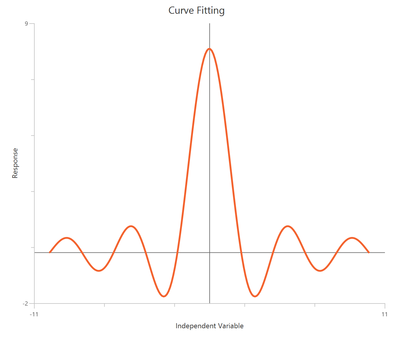
Input

The independent variable (X) must be on a linear scale (often time or distance). Values may be positive or negative; the model is well-defined at \(X=0\) by the special-case definition above. The dependent variable (Y) is the measured response in any consistent units.

Parameters

1. \(Amplitude\): The peak value at the center of the function (in Y units). By definition, \(Y(0)=Amplitude\).

2. \(Wavelength\): he characteristic period of the underlying sine term (same units as X). Smaller \(Wavelength\) produces more closely spaced oscillations.

---

Sine wave with nonzero baseline

The Sine wave with nonzero baseline model describes periodic oscillations around a constant offset rather than around zero. The waveform has constant amplitude and wavelength, but the entire curve is vertically shifted by a baseline term. This model is appropriate when the oscillatory signal fluctuates around a steady background level rather than zero.

Equation

\begin{equation} Y = Amplitude \cdot \sin\!\left(\frac{2\pi X}{Wavelength} + PhaseShift\right) + Baseline \end{equation}

Visualization

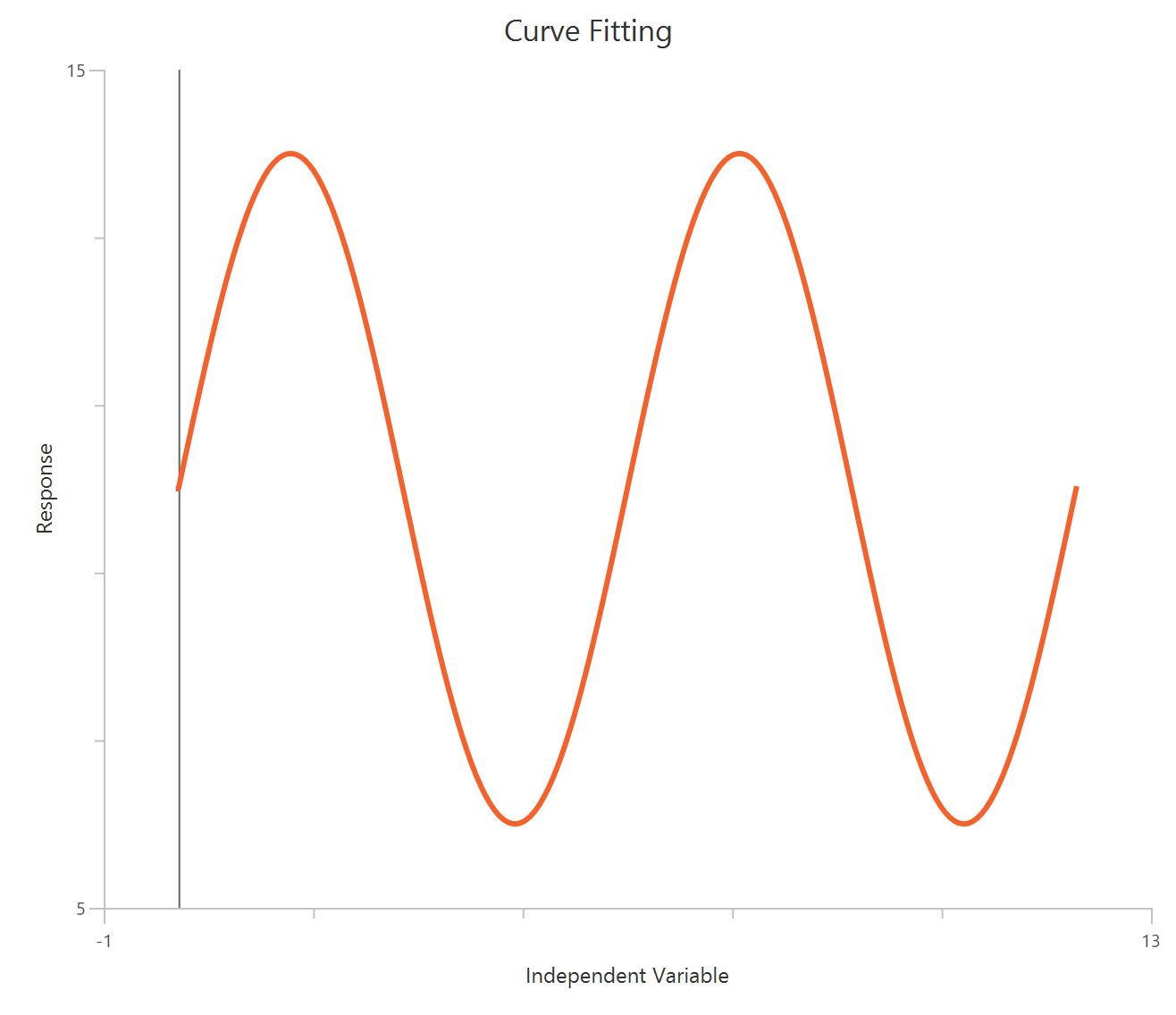
Input

The independent variable (X) must be on a linear scale (often time or distance). Values may be positive or negative; the model is well-defined at \(X=0\) by the special-case definition above. The dependent variable (Y) is the measured response in any consistent units.

Parameters

1. \(Amplitude\): The peak value at the center of the function (in Y units). By definition, \(Y(0)=Amplitude\).

2. \(Wavelength\): The characteristic period of the underlying sine term (same units as X). Smaller \(Wavelength\) produces more closely spaced oscillations.

3. \(PhaseShift\): The horizontal phase offset, expressed in radians.

4. \(Baseline\): The constant vertical offset about which the sine wave oscillates. It is expressed in the same units as Y.

---

Growth Equations

Log of exponential growth

The Log of exponential growth model is used when the response has already been logarithm-transformed. If the underlying process follows exponential growth, then plotting the logarithm of the population (or signal) versus time yields a straight line. Fitting this model is often more appropriate when measurement scatter increases with the magnitude of the response on the original scale, since the log transform can stabilize variance. For correct interpretation of doubling time, the Y values should be the natural logarithm of the population (or signal).

Equation

\begin{equation} Y = \log(Y_0) + kX \end{equation}

Visualization

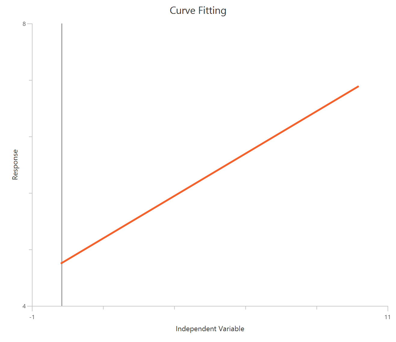
Input

The independent variable (X) is time on a linear scale (any time units). The dependent variable (Y) must be the logarithm of the measured quantity (e.g., \(Y=ln(population)\)). For meaningful doubling-time interpretation, use the natural log for Y. X values can be any real numbers; Y must be defined by your log transform (so the original, unlogged values must have been strictly positive).

Parameters

1. \(log(Y_0)\): The intercept of the line, equal to the log of the population (or signal) at \(X=0\), expressed in the same logarithmic units used for Y (typically ln units).

2. \(k\): The growth rate constant (slope), in inverse X units. Larger \(k\) corresponds to faster exponential growth on the original (unlogged) scale.

---

Logistic growth

The Logistic growth model describes population growth that is initially close to exponential but progressively slows as it approaches a maximum carrying capacity. The growth rate decreases linearly with population size, and at any time the instantaneous growth rate is proportional to \(Y(1-Y/Y_M)\), where \(Y\) is the current population and \(Y_M\) is the maximum (carrying capacity). As \(Y→Y_M\), growth slows and eventually stops.

Equation

\begin{equation} Y = \frac{Y_M \, Y_0}{(Y_M - Y_0)e^{-kX} + Y_0} \end{equation}

Visualization

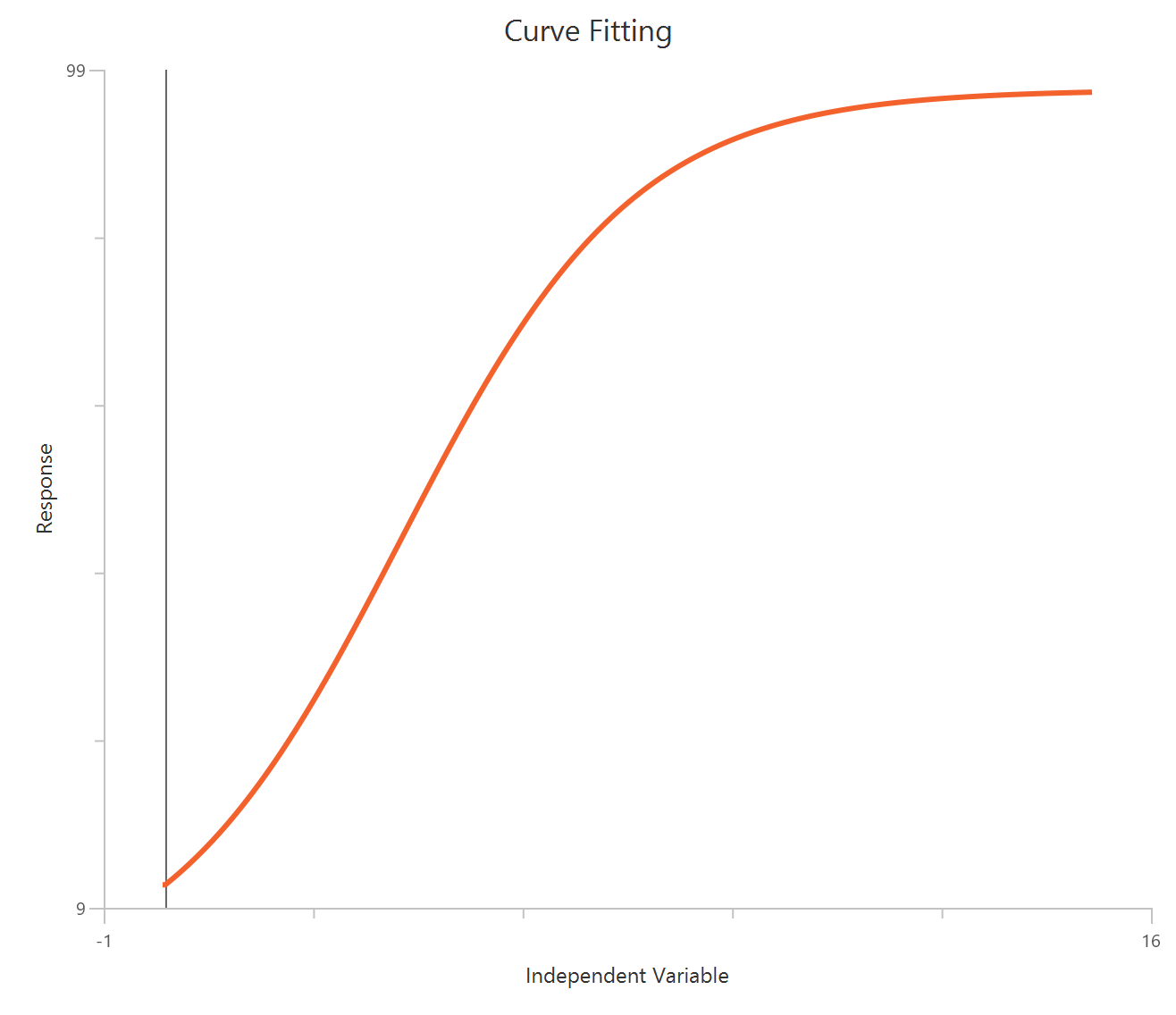
Input

The independent variable (X) represents time on a linear scale (any consistent time units). The dependent variable (Y) represents population size or another quantity that approaches a finite maximum. X values may be zero or positive. Y values must be non-negative and typically increase toward a plateau.

Parameters

1. \(Y_0\): The initial population at \(X=0\) (same units as Y).

2. \(Y_M\): The maximum population (carrying capacity), representing the asymptotic upper limit of Y (same units as Y).

3. \(k\): The logistic growth rate constant (inverse units of X). Larger \(k\) produces a steeper rise and earlier inflection.

---

Gompertz growth

The Gompertz growth model describes saturating growth where the relative growth rate decays exponentially as the population approaches its maximum. Compared with the logistic model, Gompertz growth typically rises faster when \(Y\) is small and slows more strongly near the plateau. The curve approaches an asymptote \(Y_M\) as time increases, and its inflection occurs at \(X=1/k\) under this parameterization.

Equation

\begin{equation} Y = Y_M\left(\frac{Y_0}{Y_M}\right)^{\exp(-kX)} \end{equation}

Visualization

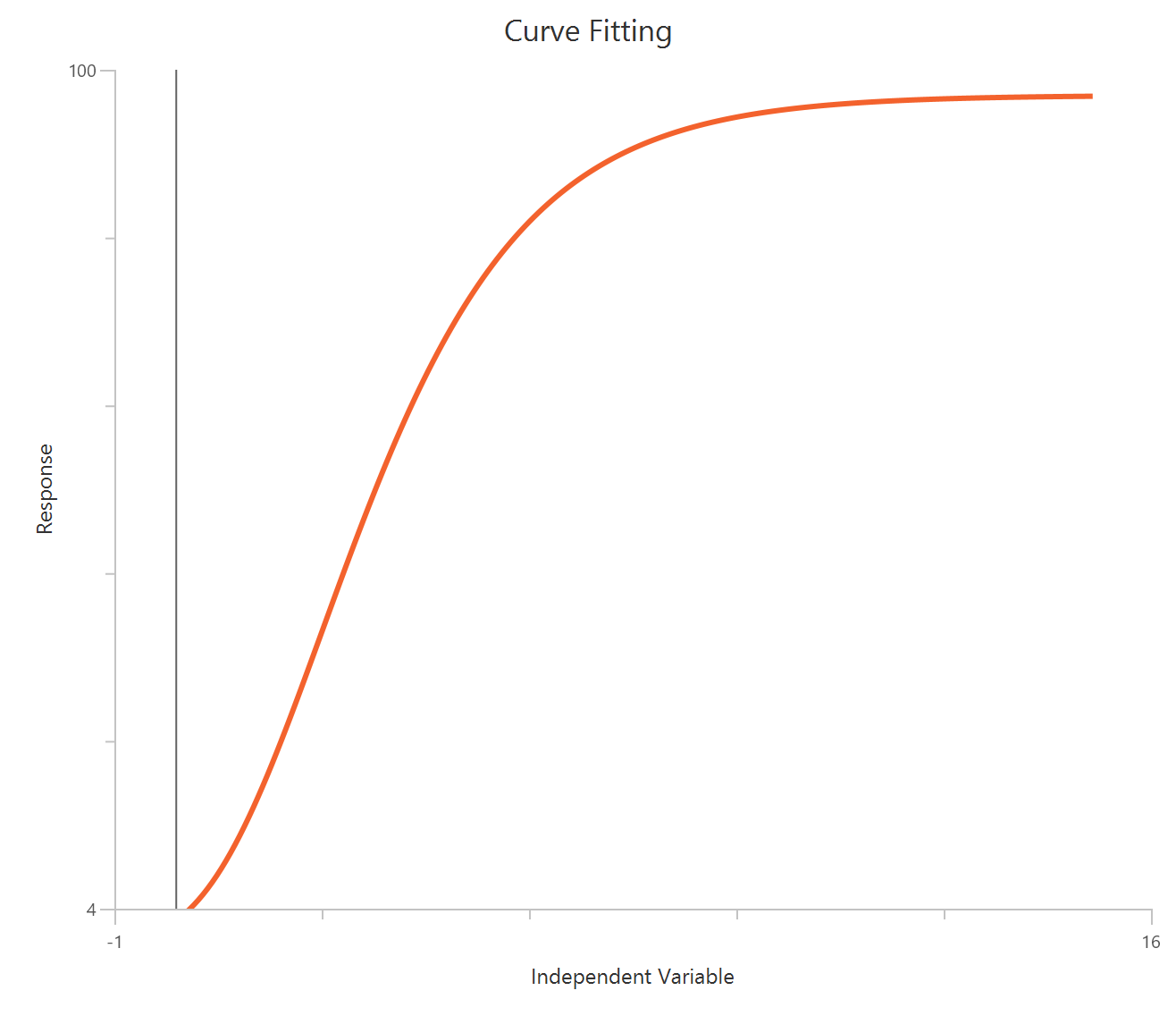
Input

The independent variable (X) represents time on a linear scale (any consistent time units). The dependent variable (Y) represents population size (or another strictly non-negative quantity) that approaches a finite maximum. X values may be zero or positive.

Parameters

1. \(Y_0\): The initial population at \(X=0\) (same units as Y).

2. \(Y_M\): The maximum population (carrying capacity), representing the asymptotic upper limit of Y (same units as Y).

3. \(k\): The Gompertz rate constant (inverse units of X). In this Prism-style parameterization,1/k is the X-value of the inflection point (often interpreted as a lag-time scale).

---

Exponential Plateau

The Exponential plateau model describes a response that starts at an initial value \(Y_0\) and rises (or falls) exponentially toward a limiting value called Plateau. The difference between the current value and the plateau decreases exponentially with rate constant k.

Equation

\begin{equation} Y = \text{Plateau} - (\text{Plateau}-Y_0)\exp(-kX) \end{equation}

Visualization

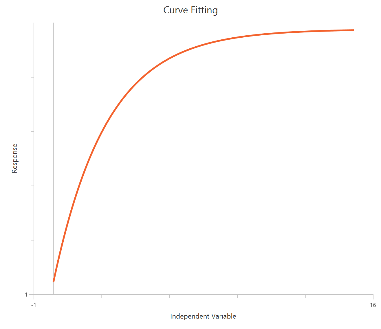
Input

The independent variable (X) must be on a linear scale and strictly positive (\(X>0\)). The model also requires a column containing the dependent variable (Y) response values (in any consistent units).

Parameters

1. \(Y_{0}\): The response at time zero (same units as \(Y\)).

2. \(Plateau\): The response at time zero (same units as \(Y\)). If background-subtracted data start at the origin, this can be fixed to 0.

3. \(k\): The rate constant (inverse units of X) that determines how quickly the curve approaches the plateau. Larger k produces a faster approach.

---

Beta growth and decline

The Beta growth and decline model describes a population (or signal) that increases from zero, reaches a single peak, and then declines back to zero by a specified end time. It is a convenient empirical model for “rise-and-fall” trajectories where you know (or can estimate) the time of the peak and the time the response returns to baseline. The curve is parameterized so that the maximum value is \(Y_m\), it peaks at time \(T_e\), and its inflection point occurs at time \(T_m\).

Equation

\begin{equation} Y = Y_m\left(1+\frac{(T_e-X)(T_e-T_m)}{X\,T_e}\right)\left(\frac{X}{T_e}\right)^{\left(\frac{T_e}{T_e-T_m}\right)} \end{equation}

Visualization

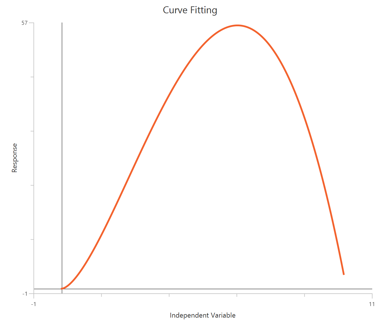
Input

The independent variable (X) is time on a linear scale. For the model to be well-defined, X values used for fitting must satisfy: \(0<X<T_e\). The dependent variable (Y) is the measured population/response in consistent units. Because the model starts and ends at zero, it is most appropriate when the response is near zero at the beginning and near zero again by \(X=T_e\) (or when data have been baseline-corrected).

Parameters

1. \(Y_m\): The peak (maximum) value of the response, in the same units as \(Y\).

2. \(T_e\): The time at which the response peaks (and the endpoint that sets the return-to-zero behavior), in the same units as \(X\). Must be positive.

3. \(T_m\): The time of the inflection point (where curvature changes sign on the rising phase), in the same units as \(X\). Must satisfy \(O<T_m<T_e\).

---

Linear–quadratic survival models

Linear Quadratic, Y is Fraction Surviving

The linear–quadratic (LQ) model describes the fraction of cells surviving after exposure to ionizing radiation. It assumes that cell killing arises from two components: a linear component proportional to dose (single-track events) and a quadratic component proportional to dose squared (interaction of sublethal damage). The model predicts a continuously decreasing survival fraction with increasing radiation dose and is widely used in radiobiology and radiation oncology.

Equation

\begin{equation} Y = \exp\left[-\left(A X + B X^{2}\right)\right] \end{equation}

Visualization

Input

The independent variable (X) represents radiation dose and must be on a linear scale with \(X \geq 0\). The dependent variable (Y) represents the fraction of cells surviving and must satisfy \(0 \leq Y \leq 1\).

Parameters

1. \(A\): The linear killing coefficient (units of inverse dose). It represents cell death caused by single radiation tracks. Larger A results in steeper initial decline in survival.

2. \(B\): The quadratic killing coefficient (units of inverse dose squared). It represents cell death from interaction of two sublethal events. Larger B increases curvature at higher doses.

---

Linear Quadratic, Y is Percent Surviving

This linear–quadratic (LQ) variant models percent cell survival after radiation exposure. As in the standard LQ model, survival decreases with dose due to a linear (single-track) and a quadratic (two-track) killing component. The only difference from the “fraction surviving” form is a scaling by 100 so that the predicted response is expressed as a percentage, approaching 100% at dose zero and decreasing toward 0% as dose increases.

Equation

\begin{equation} Y = 100 \, \exp\left[-\left(A X + B X^{2}\right)\right] \end{equation}

Visualization

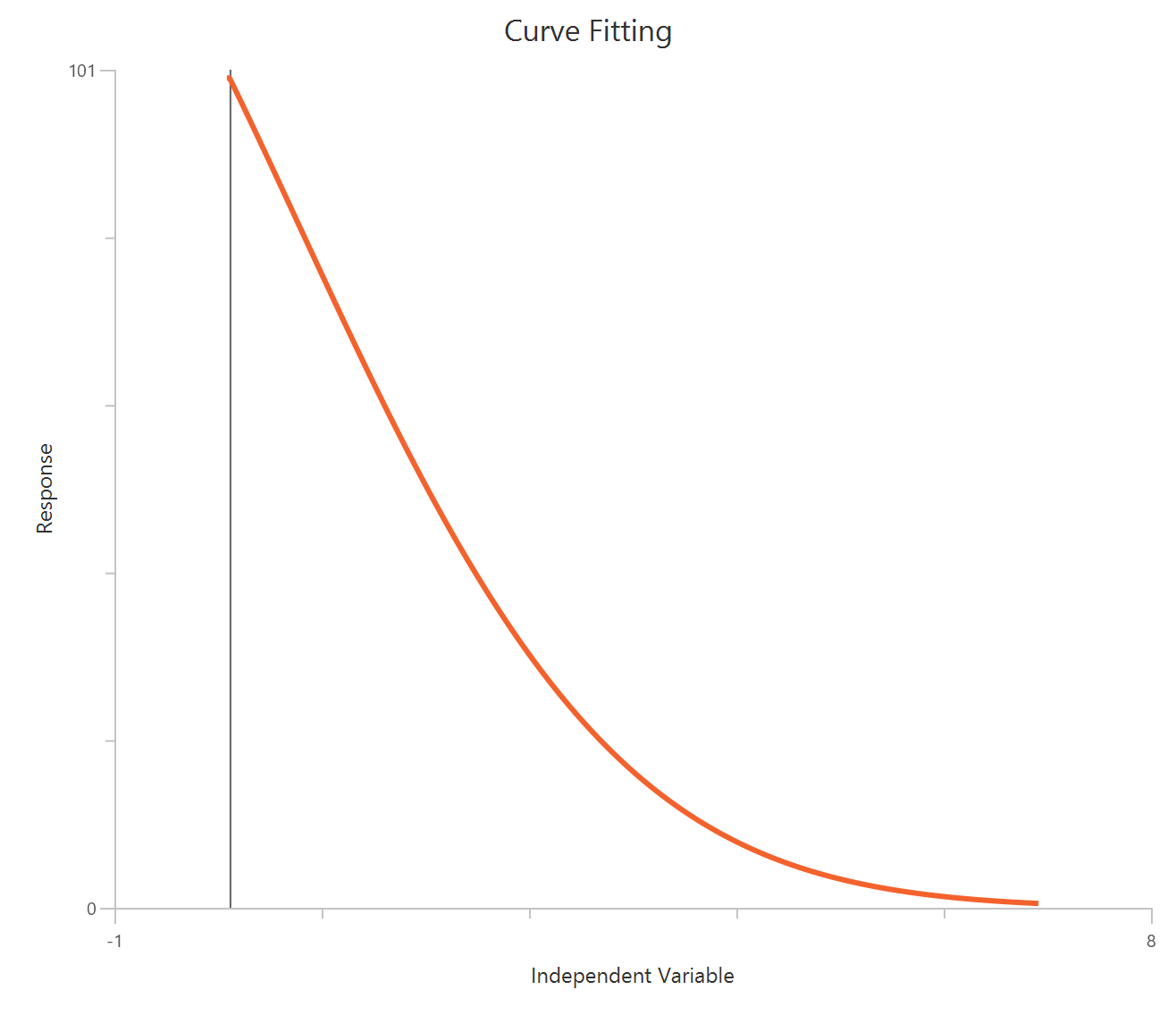
Input

The independent variable (X) represents radiation dose and must be on a linear scale with \(X \geq 0\). The dependent variable (Y) represents the fraction of cells surviving and must satisfy \(0 \leq Y \leq 100\). Y must be entered as a percentage (not a fraction). If your data are fractions, use the “fraction surviving” form instead.

Parameters

1. \(A\): The linear killing coefficient (units of inverse dose). It represents cell death caused by single radiation tracks. Larger A results in steeper initial decline in survival.

2. \(B\): The quadratic killing coefficient (units of inverse dose squared). It represents cell death from interaction of two sublethal events. Larger B increases curvature at higher doses.

---

Linear Quadratic, Y is Number Surviving

This linear–quadratic (LQ) model describes the absolute number of surviving cells after exposure to radiation dose \(X\). Survival decreases with dose according to a linear (single-event) and quadratic (two-event) killing component. Unlike the fraction or percent forms, this formulation includes an explicit initial population term \(Y_0\). ​

, which represents the number of cells present at zero dose. The model predicts exponential decay of the population size as radiation dose increases.

Equation

\begin{equation} Y = Y_0 \, \exp\left[-\left(A X + B X^{2}\right)\right] \end{equation}

Visualization

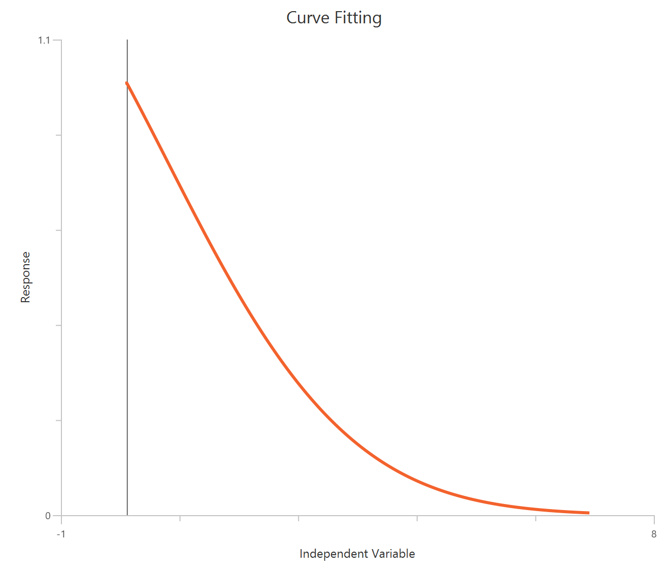
Input

The independent variable (X) must be radiation dose on a linear scale and must satisfy \(X≥0\). The dependent variable (Y) must be the number of surviving cells (absolute counts) and should be strictly positive \(Y>0\). If your data are recorded as fraction surviving or percent surviving, use the corresponding linear–quadratic model variants for those output types instead.

Parameters

1. \(Y_0\): The number of cells when \(X=0\) (initial population size), in the same units as \(Y\).

2. \(A\): The linear killing coefficient (units of inverse dose). It represents cell death caused by single radiation tracks. Larger A results in steeper initial decline in survival.

3. \(B\): The quadratic killing coefficient (units of inverse dose squared). It represents cell death from interaction of two sublethal events. Larger B increases curvature at higher doses.

---

Linear Quadratic, Y is Fraction Dead

The linear–quadratic (LQ) model describes the fraction of cells that are dead after exposure to ionizing radiation. It assumes that cell killing arises from two components: a linear component proportional to dose (single-track events) and a quadratic component proportional to dose squared (interaction of sublethal damage). The model predicts a continuously increasing death fraction with increasing radiation dose and is widely used in radiobiology and radiation oncology.

Equation

\begin{equation} Y = 1.0 - \exp\left[-\left(A X + B X^{2}\right)\right] \end{equation}

Visualization

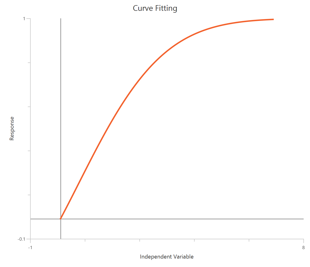
Input

The independent variable (X) represents radiation dose and must be on a linear scale with \(X \geq 0\). The dependent variable (Y) represents the fraction of cells that are dead and must satisfy \(0 \leq Y \leq 1\).

Parameters

1. \(A\): The linear killing coefficient (units of inverse dose). It represents cell death caused by single radiation tracks. Larger A results in steeper initial increase in deaths.

2. \(B\): The quadratic killing coefficient (units of inverse dose squared). It represents cell death from interaction of two sublethal events. Larger B increases curvature at higher doses.

---

Linear Quadratic, Y is Percent Dead

This linear–quadratic (LQ) variant models percent cell that are dead after radiation exposure. As in the standard LQ model, survival decreases with dose due to a linear (single-track) and a quadratic (two-track) killing component. The only difference from the “fraction dead form is a scaling by 100 so that the predicted response is expressed as a percentage, approaching 100% at dose zero and decreasing toward 0% as dose increases.

Equation

\begin{equation} Y = 100* (1.0 - \exp\left[-\left(A X + B X^{2}\right)\right]) \end{equation}

Visualization

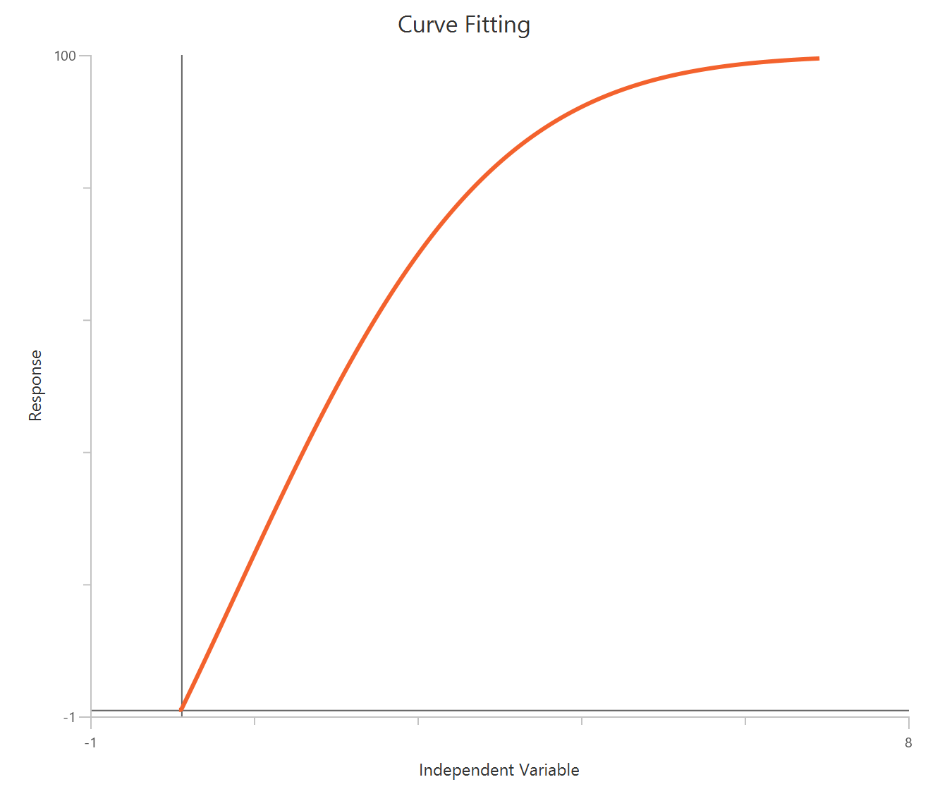
Input

The independent variable (X) represents radiation dose and must be on a linear scale with \(X \geq 0\). The dependent variable (Y) represents the fraction of cells that are dead and must satisfy \(0 \leq Y \leq 100\). Y must be entered as a percentage (not a fraction). If your data are fractions, use the “fraction dead form instead.

Parameters

1. \(A\): The linear killing coefficient (units of inverse dose). It represents cell death caused by single radiation tracks. Larger A results in steeper initial increase in death.

2. \(B\): The quadratic killing coefficient (units of inverse dose squared). It represents cell death from interaction of two sublethal events. Larger B increases curvature at higher doses.

---

Linear Quadratic, Y is Number Dead

This linear–quadratic (LQ) model describes the absolute number of dead cells after exposure to radiation dose \(X\). Deaths increase with dose according to a linear (single-event) and quadratic (two-event) killing component. Unlike the fraction or percent forms, this formulation includes an explicit initial population term \(Y_0\). , which represents the number of cells present at zero dose.

Equation

\begin{equation} Y = Y_0 * (1.0 - \exp\left[-\left(A X + B X^{2}\right)\right]) \end{equation}

Visualization

Input

The independent variable (X) must be radiation dose on a linear scale and must satisfy \(X≥0\). The dependent variable (Y) must be the number of dead cells (absolute counts) and should be positive \(Y>=0\). If your data are recorded as fraction dead or percent dead, use the corresponding linear–quadratic model variants for those output types instead.

Parameters

1. \(Y_0\): The number of cells when \(X=0\) (initial population size), in the same units as \(Y\).

2. \(A\): The linear killing coefficient (units of inverse dose). It represents cell death caused by single radiation tracks. Larger A results in steeper initial increase in deaths.

3. \(B\): The quadratic killing coefficient (units of inverse dose squared). It represents cell death from interaction of two sublethal events. Larger B increases curvature at higher doses.

---

Lethal Concentration/Dose (LCx/LDx)

In this context, LCx/LDx analysis refers to estimating the concentration (LCx) or dose (LDx) that produces a specified proportion \(x%\) of “response” (typically mortality) in a population. Unlike the nonlinear least-squares models above, LCx/LDx models are naturally formulated as a binomial-response problem: each observation represents \(y_i\) affected individuals out of \(n_i\) tested at a given concentration/dose \(X_i\). The probability of response, \(p_i\), is modeled using a generalized linear model (GLM) with a probit link:

\[ \begin{equation} y_i \sim \mathrm{Binomial}(n_i, p_i) \end{equation} \]

\[ \begin{equation} \Phi^{-1}(p_i)=\eta_i=\beta_0+\beta_1\,g(X_i) \end{equation} \]

where \(\Phi^{-1}(\cdot)\) is the inverse standard normal CDF (the probit link), \(\eta_i\) is the linear predictor, \(\beta_0,\beta_1\) are regression coefficients, and \(g(X)\) is the chosen predictor scale (commonly \(\log_{10}(X)\) for dose/concentration–response).

Once \(\beta_0\) and \(\beta_1\) are estimated, the LCx/LDx value is obtained by solving for the \(X\) that yields \(p = x/100\). Let \(z_x = \Phi^{-1}(x/100)\). Then:

\[ \begin{equation} z_x=\beta_0+\beta_1\,g(LC_x)\quad\Rightarrow\quad g(LC_x)=\frac{z_x-\beta_0}{\beta_1} \end{equation} \]

and \(LC_x\) (or \(LD_x\)) is found by applying the inverse of \(g(\cdot)\) (e.g., exponentiating if \(g(X)=\log_{10}(X)\)). This framework is preferred for lethal endpoints because it explicitly models probabilities, respects the 0–1 bounds, and correctly handles the fact that variance depends on \(p_i\) and \(n_i\), rather than assuming constant-variance residuals.

To fit probit GLMs, Isalos uses the generalized linear model routine with parameters estimated by the Newton–Raphson method. Newton–Raphson updates the coefficient vector by repeatedly using the gradient and curvature of the log-likelihood to move toward the maximum-likelihood solution. This approach is standard for GLMs because it is efficient, converges rapidly for well-behaved datasets, and provides the estimated coefficient covariance matrix needed for uncertainty quantification.

After fitting, uncertainty can be reported either on the regression coefficients or directly on derived quantities such as LC50/LD50. Symmetrical confidence intervals are computed from the approximate normality of the maximum-likelihood estimates (Wald-type intervals).

Fit your data using the Lethal Concentration/Dose (LCx/LDx) function by browsing in the top ribbon:

Statistics \(\rightarrow\) Curve Fitting \(\rightarrow\) Lethal Concentration/Dose (LCx/LDx)

Input

Numerical values should be specified in the input datasheet. The design for Lethal Concentration/Dose (LCx/LDx) requires at least three numerical columns in the input sheet: one column representing the independent variable, one column corresponding to the number of trials performed with the specified concentration/dose and one column with the number of successes. Columns with empty cells cannot be inculded in the analysis. Each row represents a single observation.

Configuration

Concentration/Dose Column	Select the column that contains the independent variable (applied concentration or dose).
Trials Column	Select the column that indicates the total number of individuals/units tested at each concentration or dose.
Successes Column	Select the column that indicates the number of observed lethal responses at each concentration or dose.
Logarithmize Concentration/Dose Column	Enable this option to transform the concentration/dose values using a base-10 logarithm, which is commonly used to stabilize variance and linearize the probit relationship.
Logarithm Base	Choose the base used for the logarithmic transformation of the concentration/dose column (default is base 10).
Lethal Effect (%)	Specify the target effect level (e.g., 50% for LC50/LD50) for which the corresponding concentration or dose will be estimated.
Confidence Level (%)	Specify the confidence level of the analysis. Values should range from 0 to 100 and correspond to percentages.

Output

The output spreadsheet contains three tables:

1. Lethal Concentration/Dose Estimation Table: contains the estimate for the lethal concentration/dose at the specified user percentage alongside its confidence interval.
2. Parameter Estimates Table: includes the estimated coefficients. Each row corresponds to a predictor and includes its coefficient, standard error, confidence interval, test statistic, degrees of freedom, and p-value.
3. Goodness of Fit: includes statistical measures that assess how well the model fits the data, such as Deviance, Log-Likelihood, AIC, BIC, and related metrics.

In addition, a pop-up window displays a plot of the fitted curve overlaid with the experimental data points.

Example

Input

In the input datasheet the requirement is to specify at least three numerical columns and insert the appropriate data, as shown below.

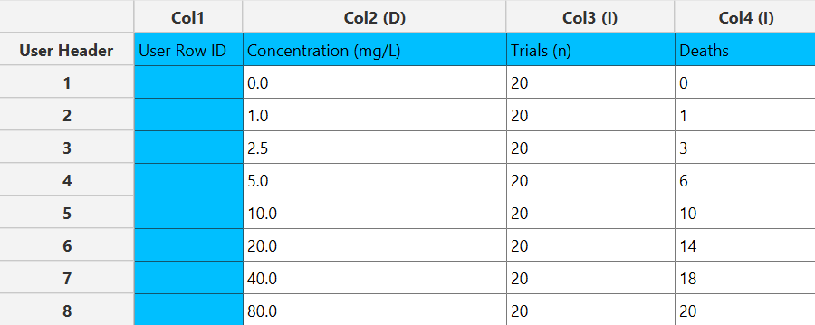
Configuration

1. Select Statistics → Curve Fitting → Lethal Concentration/Dose (LCx/LDx).
2. Select the column that corresponds to the Concentration/Dose Column[1].
3. Select the column that corresponds to the Trials Column[2].
4. Select the column that corresponds to the Successes Column[3].
5. Select/tick if you wish to Logarithmize Concentration/Dose Column before fitting [4].
6. If the logaritmize option is selected, specify the Logarithm Base[5] for the transformation.
7. Specify the Lethal Effect Level (%)[6] for which the corresponding concentration or dose will be estimated.
8. Specify the Confidence Level (%)[7] for tests.
9. Click on the Execute button [8] to perform the Non Linear Curve Fitting method.

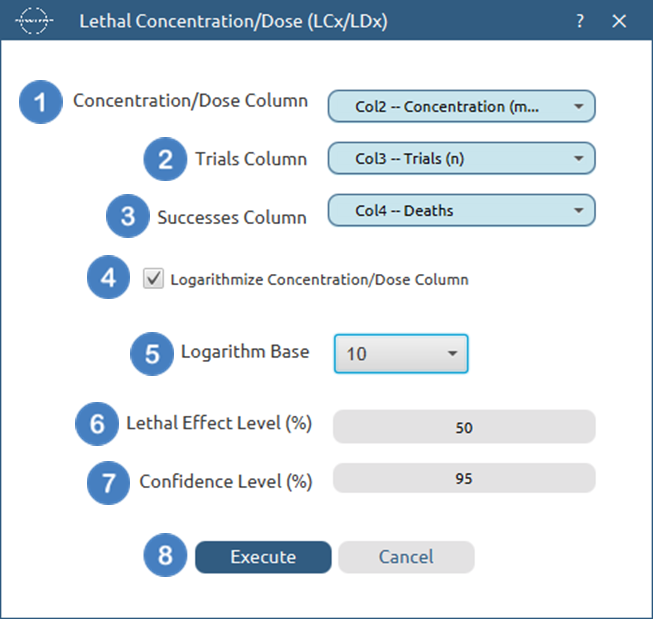
Output

The lethal concentration/dose estimates, parameter estimates and goodness of fit tables are shown in the output spreadsheet and the line chart showcasing the fitted curve and the experimental points is shown in a separate window.

---

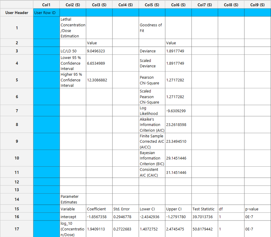
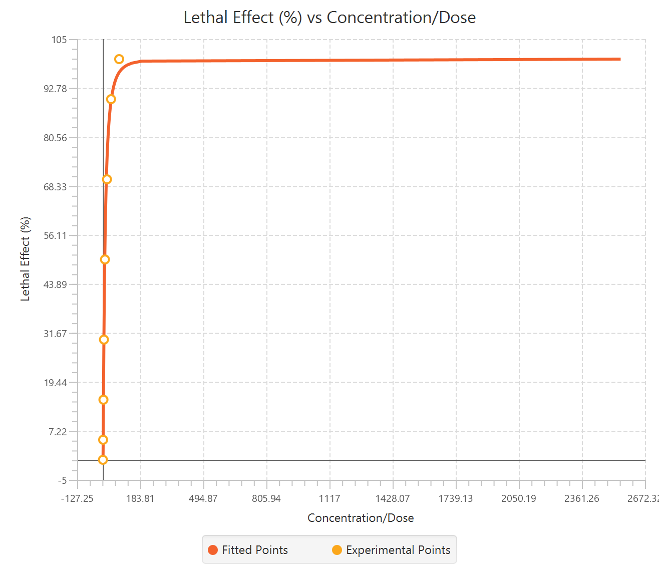
References

1. Vetterling, William T., and William H. Press. Numerical recipes: example book C. Cambridge University Press, 1992.
2. Glantz, Stanton A., Bryan K. Slinker, and Torsten B. Neilands. “Primer of applied regression & analysis of variance.” (No Title) (1990).

---

Version History

Introduced in Isalos Analytics Platform v2.1.0

Instructions last updated on January 2025