Survival Analysis
Survival Analysis, also known as “Time-to-Event” data analysis, is a collectuib of statistical methods that are used for analyzing data mesauring time until an event of interest occurs. Typical examples of such events include death, onset of disease, system failure, or arrival times. These methods are particularly useful when the timing of the event is as important as whether the event occurs.
A defining characteristic of survival data is that it is often incomplete, meaning that for some observations the event of interest is not observed within the study period. This gives rise to concepts such as censoring and truncation, which must be properly handled to avoid biased results.
Censoring
Censoring occurs when the exact event time is not known, but partial information about it is available. Survival analysis methods are specifically designed to incorporate censored observations without discarding them.
The main types of censoring are:
- Right Censoring: The most common form. The event has not occurred by the end of the observation period or the subject is lost to follow-up. Example: A patient is still alive at the end of a clinical trial.
- Left Censoring: The event has already occurred before the subject enters the study, but the exact time is unknown. Example: A disease is detected at diagnosis, but the onset time is unknown.
- Interval Censoring: The event occurs within a known time interval, but the exact timing is unknown. Example: A condition is identified between two medical check-ups.
Truncation
Truncation refers to situations where certain observations are systematically excluded from the dataset based on their event times. Unlike censoring, truncated observations are not observed at all.
The main types of truncation are:
- Left Truncation (Delayed Entry): Subjects enter the study only if their event time exceeds a certain threshold. Example: Individuals are only included if they survive past a specific age.
- Right Truncation: Subjects are only observed if the event has already occurred before a certain cutoff. Example: Studying only individuals who have already experienced failure before a given time.
Proper handling of truncation is essential, as ignoring it can lead to significant selection bias.
Key Functions in Survival Analysis
Survival analysis is built around several fundamental functions that describe the distribution of time-to-event data:
- Survival Function \(S(t)\): The survival function represents the probability that the event of interest has not occurred by time \(t\): $$ \begin{equation} S(t) = P(T > t) \end{equation} $$
- Probability Density Function \(f(t)\): Describes the instantaneous likelihood of the event occurring at time \(t\).
- Cumulative Distribution Function \(F(t)\): Represents the probability that the event has occurred by time \(t\): $$ \begin{equation} F(t) = P(T \leq t) = 1 - P(T > t) = 1 - S(t) \end{equation} $$
- Hazard Function \(h(t)\): The hazard function represents the instantaneous rate at which events occur at time \(t\), given survival up to that time: $$ \begin{equation} h(t) = lim_{\Delta t \rightarrow 0} \frac{P(t<T<\Delta t | T \geq t)}{\Delta t} \end{equation} $$
It provides insight into the risk dynamics over time.
- Cumulative Hazard Function \(H(t)\): Defined as the accumulated hazard over time: $$ \begin{equation} H(t) = \int_0^t h(u) du \end{equation} $$
It is related to the survival function via:
$$ \begin{equation} S(t) = e^{-H(t)} \end{equation} $$
The above functions are equivalent ways to describe a continuous probability distribution.
Non-Parametric Methods
Non-parametric methods in survival analysis are statistical techniques that estimate survival characteristics without assuming any specific underlying probability distribution for the time-to-event data. This makes them particularly flexible and widely applicable, especially in exploratory analysis or when the true distribution of the data is unknown.
These methods rely directly on the observed data to construct estimates of key functions such as the survival function and, in some cases, the hazard function. Because they do not impose distributional assumptions, they are generally more robust but may be less efficient than parametric approaches when the underlying distribution is known.
Non-parametric methods are primarily used to:
- Estimate the survival function \(S(t)\) from observed data
- Incorporate censored observations naturally into the analysis
- Provide descriptive insights into survival patterns over time
- Compare survival experiences between different groups These methods are often the first step in survival analysis, offering a data-driven overview before applying more complex modeling techniques.
Kaplan-Meier Estimator
The Kaplan–Meier estimator is a non-parametric method used to estimate the survival function from time-to-event data. It incorporates information from all available observations—both uncensored (events) and right-censored—by constructing the survival function as a sequence of stepwise estimates at observed event times.
Rather than treating time as continuous, the method partitions the time axis into intervals defined by the ordered distinct event times. At each event time \(t_i\), the survival probability is updated based on the observed data.
At each event time \(t_i\), the Kaplan–Meier estimator computes the conditional probability of surviving past that time as:
where:
- \(d_i\) is the number of events occuring at time \(t_i\).
- \(n_i\) is the number of individuals at risk just prior to time \(t_i\).
The survival function is then estimated as the product of these conditional probabilities up to time \(t\):
With the estimate being initialized with \(S(0) = 1\).
Right-censored observations are naturally incorporated into the Kaplan–Meier estimation process by contributing to the risk set up until the time at which they are censored. At each event time, the number of individuals at risk includes all subjects who have neither experienced the event nor been censored prior to that time. Once a subject becomes censored, they are removed from the risk set for all subsequent time points and no longer contribute to the calculation of survival probabilities. Importantly, censored observations do not count as events and therefore do not directly cause decreases in the survival function. Instead, their impact is indirect, as they reduce the number of individuals at risk in future intervals, which in turn influences the magnitude of subsequent survival probability estimates.
The Kaplan–Meier estimator produces a survival function that takes the form of a right-continuous step function, where changes in the estimated survival probability occur only at observed event times. Between these times, the survival probability remains constant. When multiple events occur at the same time point, they are handled collectively by aggregating them into a single step, ensuring that the calculation properly reflects the number of events relative to the individuals at risk. As a non-parametric method, the Kaplan–Meier estimator does not rely on any assumptions regarding the underlying distribution of survival times; instead, the shape of the survival curve is determined entirely by the observed data. This data-driven nature makes the estimator highly flexible and widely applicable, although it also limits its ability to extrapolate beyond the range of observed time points.
The variability of the survival estimate is commonly assessed using Greenwood’s formula, which provides an estimate of the variance:
From this, the standard error can be derived, allowing the construction of confidence intervals for the survival function.
The results of the Kaplan–Meier estimator are visualized using the Kaplan–Meier survival curve, which displays the estimated survival probability over time and confidence intervals, shown as bands around the curve. The median survival time is can be derived directly from the curve as the time at which \(S(t) \leq 0.5\). Optionally the user can select to visualize the estimated hazard function and the estimated cumulative probability of failure.
Use the Kaplan Meier Estimator method by browsing in the top ribbon:
Statistics \(\rightarrow\) Survival Analysis \(\rightarrow\) Non-Parametric \(\rightarrow\) Kaplan Meier Estimator |
Input
The Kaplan–Meier estimator requires at least one column of numerical data to be specified in the input datasheet. The required input is a time variable column containing non-negative numerical values, representing the observed time-to-event or time-to-censoring for each subject. In addition to the time variable, several optional inputs may be provided to extend the functionality of the analysis. A censoring column may be specified as a variable, either numerical or textual, indicating whether each observation corresponds to an event or a censored case. A frequency column may also be included, consisting of non-negative numerical values that represent the number of identical observations associated with each row; if this column is not provided, each row is treated as a single observation by default. Furthermore, an event mode column may be defined, which can be either numerical or textual, and is used to distinguish between different types of events depending on the analysis configuration. Finally, a grouping column can be specidied as a categorical variable, either numerical or textual, indicating the group membership of each observation. All input columns must be of consistent type and should not contain invalid or missing values, as this may prevent the method from executing correctly.
Configuration
| Time Column | Select the column corresponding to the observed time-to-event or time-to-censoring for each subject. This column must be numerical and contain non-negative values. |
| Configure Event Mode Options | Use this button to open the Configure Event Mode Options window |
| Event Mode Column | Within the Configure Event Mode Options window, specify the column containing event mode information. |
| Levels not Considered as Event/Levels Considered as Event | Manually select which levels should be treated as events from the available levels of the Event Mode Column. Use the arrow buttons to move levels between the two lists. Single-arrow buttons move selected levels, while double-arrow buttons move all levels. At least one level must be selected as an event. |
| Clear Event Mode Options | Use this button to clear all selections related to event mode configuration. |
| Use a Frequency Column | Enable this option to include a frequency column in the analysis. |
| Frequency Column | If the Use a Frequency Column option is enabled, select the column containing frequency information for each observation. This column must be numerical and contain non-negative values. |
| Use a Censoring Column | Enable this option to include a censoring column in the analysis. |
| Censoring Column | If the Use a Censoring Column option is enabled, select the column containing censoring information for each observation. This column must be categorical and may be either numerical or textual. |
| Censoring Indicator Value | If a censoring column is used, specify which of its two levels represents a censored observation. |
| Censor times at or above a value | Enable this option to treat all time values greater than or equal to a specified threshold as censored. |
| Censoring Threshold Value | If the Censor times at or above a value option is enabled, specify the value above or equal to which observations will be treated as censored. |
| Use a Grouping Column | Enable this option to include a grouping column in the analysis, allowing comparison of survival across different groups in the population. |
| Grouping Column | If the Use a Grouping Column option is enabled, select the column containing grouping information for each observation. This column must be categorical. |
| Confidence Level (%) | Specify the confidence level of the analysis. Values should range from 0 to 100 and correspond to percentages. Default value is set to 95. |
| Confidence Interval Type | Select the type of confidence interval to compute. Available options include: Two-sided, Lower Bound, Upper Bound. |
| Hazard Function Plot | Enable this option to generate a plot of the estimated hazard function over time. |
| Cumulative Probability of Failure Plot | Enable this option to generate a plot of the estimated cumulative probability of failure over time. |
Output
The output spreadsheet contains a table summarizing the survival analysis results at each observed time point. This includes the number of subjects at risk, the number of events, the estimated survival probability, its standard error, and the corresponding confidence interval bounds at the selected confidence level. If a grouping column is specified, the spreadsheet first presents the overall results for the full sample, followed by separate tables for each group. In addition, a pop-up window displays the Kaplan–Meier survival curve, showing the stepwise estimate of survival probability over time along with the associated confidence interval bounds. When grouping is enabled, the plot includes the overall survival curve as well as separate curves with confidence bounds for each group. Similarly, if selected, the hazard function and cumulative probability of failure plots are generated and display both the overall estimates and the corresponding group-specific curves.
Example
Input
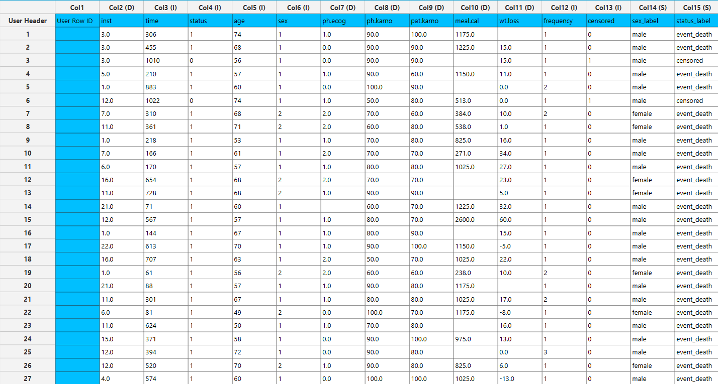
In the input datasheet the requirement is to specify at least one numerical column and insert the appropriate data, as shown below.
Configuration
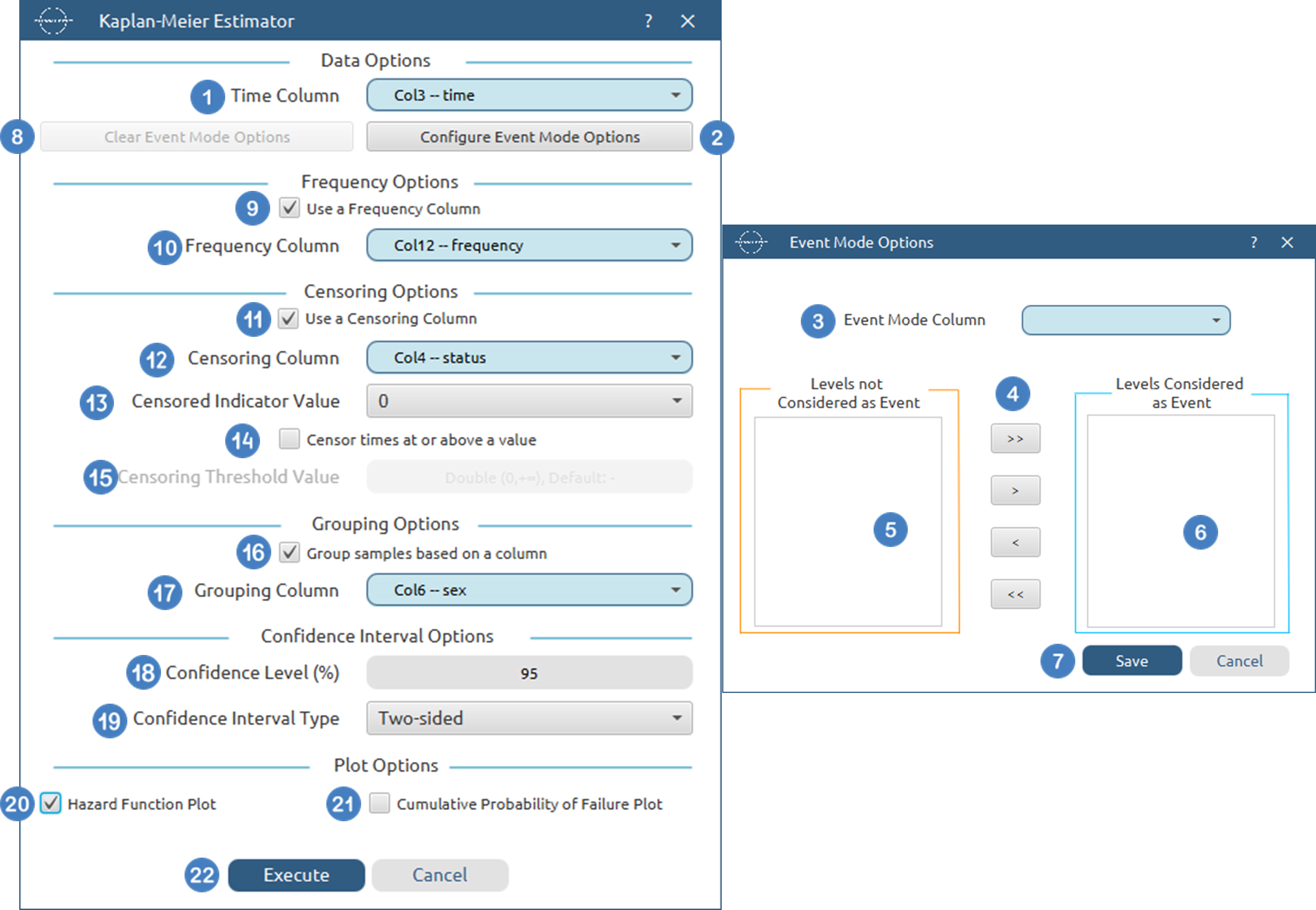
- Select
Statistics→Survival Analysis→Non-Parametric→Kaplan-Meier Estimator. - Select the
Time Column[1]. This column should contain non-negative numeric values. - Optionally click on the
Configure Event Mode Options[2] button to select anEvent Mode Column[3] and use the arrow buttons [4] to select the levels that should be accounted for in the analysis by moving them between theLevels not Considered as Event[5] andLevels Considered as Event[6] lists.SaveorCancelany changes made using the appropriate buttons [7]. - Once you have configured some Event Mode Options you can optionally use the
Clear Event Mode Options[8] button to erase any selections made. - Select/tick to
Use a Frequency Column[9]. - If the
Use a Frequency Columnoption is selected, specify aFrequency Column[10]. This column should contain non-negative numeric values. - Select/tick to
Use a Censoring Column[11]. - If the
Use a Censoring Columnoption is selected, specify aCensoring Column[12] and the value of this column that should be theCensored Indicator Value[13]. - Select/tick to
Censor times at or above a value[14]. - If the ``Censor times at or above a value
option is selected, specify aCensoring Thresholdd Value`[15] above which events are considered censored. - Select/tick to
Use a Grouping Column[16]. - If the
Use a Grouping Columnoption is selected, specify aGrouping Column[17]. This column should be categorical, either textual or numerical. - Specify the
Confidence Level(%) [18] for Confidence Intervals and the desiredConfidence Interval Type[19]. - Optionally select/tick to calculate and present the
Hazard Function Plot[20] and theCumulative Probability of Failure Plot[21]. - Click on the
Executebutton [22] to perform the Kaplan-Meier Estimator.
Output
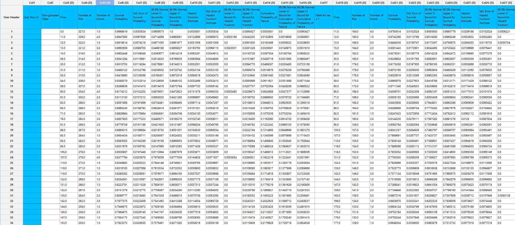
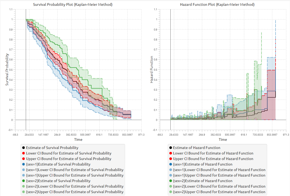
The tables summarizing the survival analysis results for the non grouped dataset and each grouping level are shown in the output spreadsheet. In addition, a pop-up window displays the Kaplan–Meier survival curve and, if selected, the hazard function and cumulative probability of failure plots.
Life Table Analysis
The Life Table method (also known as the Actuarial method) is a non-parametric approach used to estimate survival characteristics from time-to-event data by grouping observations into time intervals. Unlike the Kaplan–Meier estimator, which updates the survival estimate at each distinct event time, the Life Table method summarizes the data within predefined intervals and computes the relevant quantities at the interval level.
The time axis is partitioned into consecutive intervals of the form \([0,e_0), [e_0,e_1), ... , [e_{k-1},e_k), [e_k,\infty)\). These intervals may either be specified explicitly through user-defined endpoints or generated automatically using a given end time and interval width.
For each interval \(i\), the method determines the number of subjects entering the interval, the number of events occurring within the interval, and the number of censored observations. If a frequency column is provided, observations contribute according to their specified frequencies. Optional censoring indicators and threshold censoring are also incorporated, and event mode filtering allows only selected event types to be considered.
Because censoring may occur at any point within an interval, the method uses an effective sample size defined as
where \(n_i\) is the number of subjects entering interval \(i\) and \(w_i\) is the number censored within that interval. This adjustment reflects the assumption that censoring occurs approximately uniformly throughout the interval.
The conditional probability of failure in interval \(i\) is then estimated as
where \(d_i\) is the number of events occurring in that interval.
The survival function is estimated as the product of the conditional survival probabilities across intervals:
with the estimate initialized at \(S(0)=1\). The resulting survival curve is a step function with changes occurring at the interval boundaries.
In addition to the survival function, the method also estimates the hazard function within each finite interval. In this implementation, the hazard is computed using an exposure-based approximation, where the exposure accounts for both censoring and events within the interval. The hazard estimate therefore represents the event rate over the interval and is associated with the midpoint of the interval.
The variability of the estimates is assessed using a Greenwood-type variance formulation applied at the interval level. Standard errors are computed for the conditional probability of failure, the survival function, and the hazard function, and corresponding confidence intervals are constructed according to the selected confidence level and interval type.
The Life Table method produces a structured tabular output in which each row corresponds to an interval. For each interval, the table reports the number entering the interval, the number of events, the number censored, the effective sample size, the conditional probability of failure, the estimated survival probability at the end of the interval, and the hazard function, together with their standard errors and confidence interval bounds. The final interval is represented as an open-ended interval \([a,+∞)\); quantities that depend on a finite interval width, such as the hazard function and survival updates, are only reported for the finite intervals.
The results are typically visualized using plots of the survival function, and optionally the hazard function and cumulative probability of failure, providing a graphical representation of the interval-based estimates.
Use the Life Table Analysis method by browsing in the top ribbon:
Statistics \(\rightarrow\) Survival Analysis \(\rightarrow\) Non-Parametric \(\rightarrow\) Life Table Analysis |
Input
The Life Table method requires at least one column of numerical data to be specified in the input datasheet. The required input is a time variable column containing non-negative numerical values, representing the observed time-to-event or time-to-censoring for each subject. In addition to the time variable, several optional inputs may be provided to extend the functionality of the analysis. A censoring column may be specified as a categorical variable, either numerical or textual, indicating whether each observation corresponds to an event or a censored case. A frequency column may also be included, consisting of non-negative numerical values that represent the number of identical observations associated with each row; if this column is not provided, each row is treated as a single observation by default. Furthermore, an event mode column may be defined, which can be either numerical or textual, and is used to distinguish between different types of events depending on the analysis configuration. A grouping column may also be specified as a categorical variable, either numerical or textual, indicating the group membership of each observation. An additional optional column may be provided to specify the endpoints of the intervals used in the analysis; if this is not specified, the intervals are generated automatically based on the chosen end time and interval width. All input columns must be of consistent type and should not contain invalid or missing values, as this may prevent the method from executing correctly.
Configuration
| Time Column | Select the column corresponding to the observed time-to-event or time-to-censoring for each subject. This column must be numerical and contain non-negative values. |
| Configure Event Mode Options | Use this button to open the Configure Event Mode Options window |
| Event Mode Column | Within the Configure Event Mode Options window, specify the column containing event mode information. |
| Levels not Considered as Event/Levels Considered as Event | Manually select which levels should be treated as events from the available levels of the Event Mode Column. Use the arrow buttons to move levels between the two lists. Single-arrow buttons move selected levels, while double-arrow buttons move all levels. At least one level must be selected as an event. |
| Clear Event Mode Options | Use this button to clear all selections related to event mode configuration. |
| Specify End Time and Time Steps / Use a column to specify end points | Select whether to define the intervals automatically by specifying an end time and interval width, or to provide a column containing the endpoints of each interval. |
| Intervals through / by | Specify the end time and the width of each interval when automatic interval generation is selected. |
| End Points Column | If the option to use a column is selected, choose the column containing the endpoints of the intervals. This column must be numerical and contain non-negative values. |
| Use a Frequency Column | Enable this option to include a frequency column in the analysis. |
| Frequency Column | If the Use a Frequency Column option is enabled, select the column containing frequency information for each observation. This column must be numerical and contain non-negative values. |
| Use a Censoring Column | Enable this option to include a censoring column in the analysis. |
| Censoring Column | If the Use a Censoring Column option is enabled, select the column containing censoring information for each observation. This column must be categorical and may be either numerical or textual. |
| Censoring Indicator Value | If a censoring column is used, specify which of its two levels represents a censored observation. |
| Censor times at or above a value | Enable this option to treat all time values greater than or equal to a specified threshold as censored. |
| Censoring Threshold Value | If the Censor times at or above a value option is enabled, specify the value above or equal to which observations will be treated as censored. |
| Use a Grouping Column | Enable this option to include a grouping column in the analysis, allowing comparison of survival across different groups in the population. |
| Grouping Column | If the Use a Grouping Column option is enabled, select the column containing grouping information for each observation. This column must be categorical. |
| Confidence Level (%) | Specify the confidence level of the analysis. Values should range from 0 to 100 and correspond to percentages. Default value is set to 95. |
| Confidence Interval Type | Select the type of confidence interval to compute. Available options include: Two-sided, Lower Bound, Upper Bound. |
| Hazard Function Plot | Enable this option to generate a plot of the estimated hazard function over time. |
| Cumulative Probability of Failure Plot | Enable this option to generate a plot of the estimated cumulative probability of failure over time. |
Output
The output spreadsheet contains a table summarizing the survival analysis results for each time interval. This includes the number of subjects entering the interval, the number of events, the number censored, the effective sample size, the estimated conditional probability of failure, its standard error, and the corresponding confidence interval bounds at the selected confidence level. In addition, the table reports the estimated survivor function at the end of each interval, along with its standard error and confidence bounds, as well as the estimated hazard function and its associated uncertainty measures for finite intervals. If a grouping column is specified, the spreadsheet first presents the overall results for the full sample, followed by separate tables for each group.
In addition, a pop-up window displays the Life Table survival curve, showing the stepwise estimate of survival probability across intervals along with the associated confidence interval bounds. When grouping is enabled, the plot includes the overall survival curve as well as separate curves with confidence bounds for each group. Similarly, if selected, the hazard function and cumulative probability of failure plots are generated and display both the overall estimates and the corresponding group-specific curves.
Example
Input
In the input datasheet the requirement is to specify at least one numerical column and insert the appropriate data, as shown below.
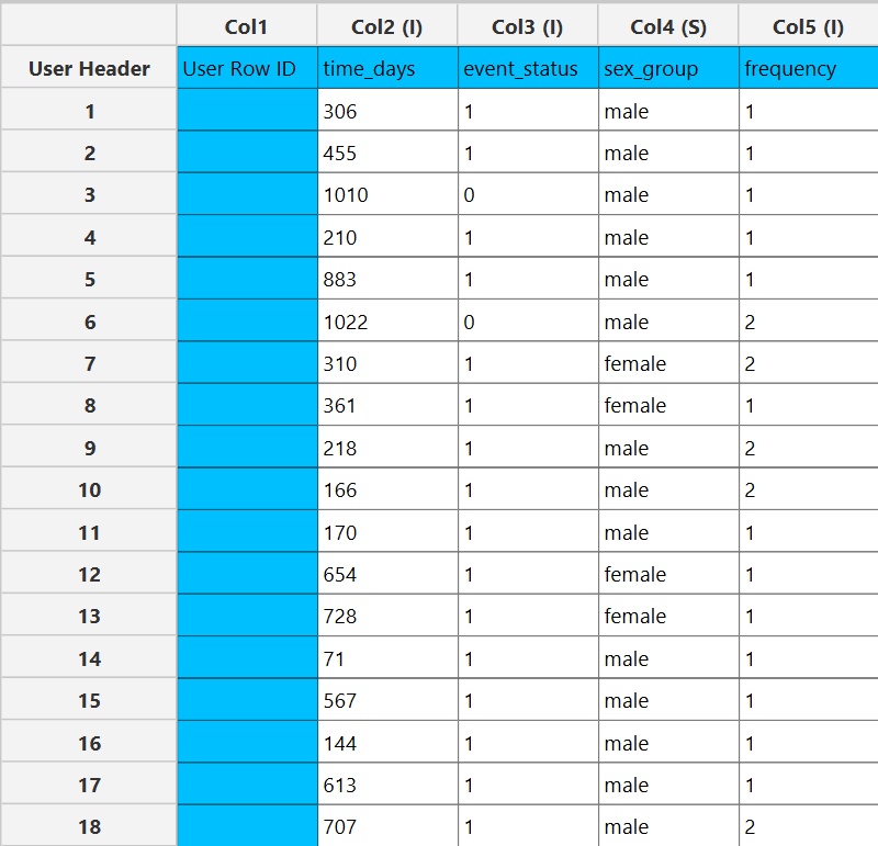
Configuration
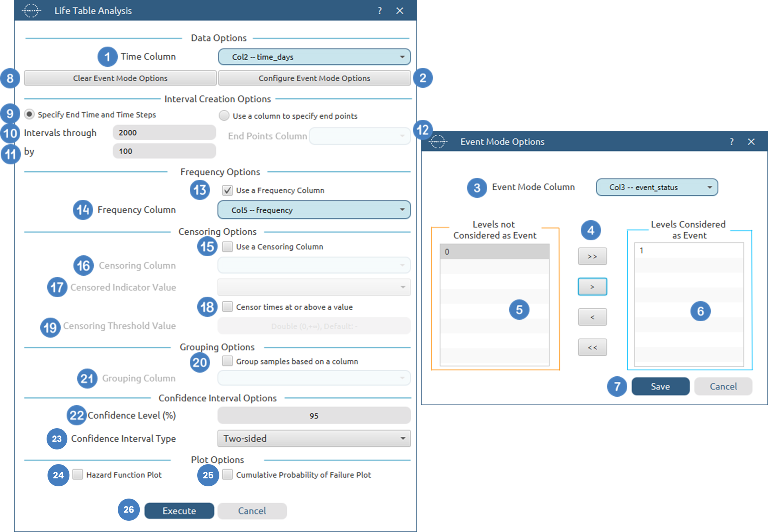
- Select
Statistics→Survival Analysis→Non-Parametric→Kaplan-Meier Estimator. - Select the
Time Column[1]. This column should contain non-negative numeric values. - Optionally click on the
Configure Event Mode Options[2] button to select anEvent Mode Column[3] and use the arrow buttons [4] to select the levels that should be accounted for in the analysis by moving them between theLevels not Considered as Event[5] andLevels Considered as Event[6] lists.SaveorCancelany changes made using the appropriate buttons [7]. - Once you have configured some Event Mode Options you can optionally use the
Clear Event Mode Options[8] button to erase any selections made. - Select whether to
Specify End Time and Time StepsorUse a column to specify end pointsfor the Interval Creation [9]. - If you choose to
Specify End Time and Time Stepsthen specify the end time[10] and the time steps [11], otherwise select theEnd Points Column[12] - Select/tick to
Use a Frequency Column[13]. - If the
Use a Frequency Columnoption is selected, specify aFrequency Column[14]. This column should contain non-negative numeric values. - Select/tick to
Use a Censoring Column[15]. - If the
Use a Censoring Columnoption is selected, specify aCensoring Column[16] and the value of this column that should be theCensored Indicator Value[17]. - Select/tick to
Censor times at or above a value[18]. - If the ``Censor times at or above a value
option is selected, specify aCensoring Thresholdd Value`[19] above which events are considered censored. - Select/tick to
Use a Grouping Column[20]. - If the
Use a Grouping Columnoption is selected, specify aGrouping Column[21]. This column should be categorical, either textual or numerical. - Specify the
Confidence Level(%) [22] for Confidence Intervals and the desiredConfidence Interval Type[23]. - Optionally select/tick to calculate and present the
Hazard Function Plot[24] and theCumulative Probability of Failure Plot[25]. - Click on the
Executebutton [26] to perform the Life-table analysis.
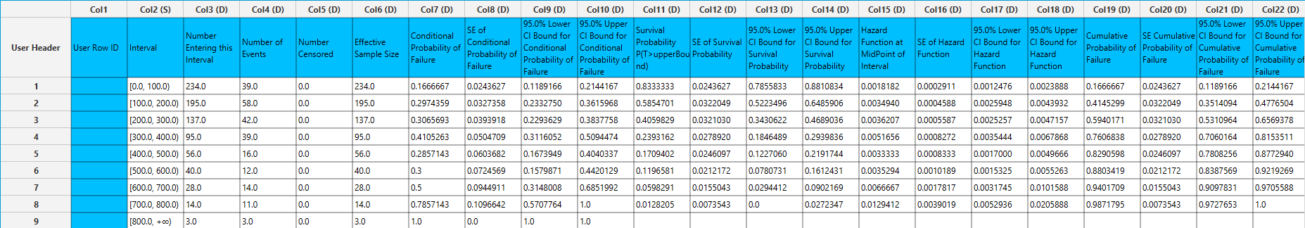
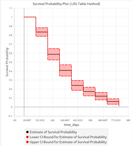
Output
The tables summarizing the survival analysis results for the non grouped dataset and each grouping level are shown in the output spreadsheet. In addition, a pop-up window displays the Life-table survival curve and, if selected, the hazard function and cumulative probability of failure plots.
Nelson-Aalen Method
The Nelson–Aalen estimator is a non-parametric method used to estimate the cumulative hazard function from time-to-event data. Unlike the Kaplan–Meier estimator, which directly estimates the survival function, the Nelson–Aalen method focuses on estimating the cumulative hazard and then derives the survival function from it.
The method operates on the ordered distinct event times. For each time point \(t_i\), the number of individuals at risk just prior to that time and the number of events occurring at that time are determined. Observations may contribute with frequency weights if a frequency column is provided, and optional censoring indicators, threshold censoring, and event mode filtering are incorporated in the same manner as in other survival methods.
At each event time \(t_i\), the hazard increment is estimated as
where \(d_i\) is the number of events occurring at time \(t_i\) and \(n_i\) is the number of individuals at risk just prior to that time.
The cumulative hazard function is then obtained by summing these increments over time:
The estimate is initialized at \(H(0)=0\) and increases in a stepwise manner at observed event times.
Right-censored observations are incorporated by contributing to the risk set up until their censoring time. At each time point, the number at risk includes all individuals who have not yet experienced the event or been censored prior to that time. After their censoring time, these observations are removed from the risk set and no longer contribute to subsequent calculations. As with other non-parametric methods, censored observations do not count as events and therefore do not directly affect the hazard increments, but they influence the estimates through their effect on the number at risk.
The Nelson–Aalen estimator produces a cumulative hazard function that is a non-decreasing step function, with jumps occurring only at observed event times. The size of each jump corresponds to the ratio of the number of events to the number at risk at that time.
The variability of the cumulative hazard estimate is assessed using the variance estimator
from which the standard error can be derived. Confidence intervals for the cumulative hazard are constructed using a normal approximation based on the selected confidence level.
The survival function is obtained from the cumulative hazard through the transformation
and the cumulative probability of failure is computed as
Confidence intervals for the survival function and cumulative probability of failure are derived by transforming the confidence bounds of the cumulative hazard estimate.
The Nelson–Aalen method produces a tabular output in which each row corresponds to a time point at which at least one event occurs. For each such time, the table reports the number at risk, the number of events, the hazard increment, the cumulative hazard estimate, and its standard error, together with the corresponding confidence interval bounds. In addition, the table includes the derived survival probability and cumulative probability of failure, along with their associated confidence intervals.
The results are typically visualized using stepwise plots of the the survival function, and optionally the cumulative probability of failure and the cumulative hazard function, providing a comprehensive view of the event dynamics over time.
Use the Nelson-Aalen Method by browsing in the top ribbon:
Statistics \(\rightarrow\) Survival Analysis \(\rightarrow\) Non-Parametric \(\rightarrow\) Nelson-Aalen Method |
Input
The Nelson-Aalen Method requires at least one column of numerical data to be specified in the input datasheet. The required input is a time variable column containing non-negative numerical values, representing the observed time-to-event or time-to-censoring for each subject. In addition to the time variable, several optional inputs may be provided to extend the functionality of the analysis. A censoring column may be specified as a categorical variable, either numerical or textual, indicating whether each observation corresponds to an event or a censored case. A frequency column may also be included, consisting of non-negative numerical values that represent the number of identical observations associated with each row; if this column is not provided, each row is treated as a single observation by default. Furthermore, an event mode column may be defined, which can be either numerical or textual, and is used to distinguish between different types of events depending on the analysis configuration. Finally, a grouping column can be specidied as a categorical variable, either numerical or textual, indicating the group membership of each observation. All input columns must be of consistent type and should not contain invalid or missing values, as this may prevent the method from executing correctly.
Configuration
| Time Column | Select the column corresponding to the observed time-to-event or time-to-censoring for each subject. This column must be numerical and contain non-negative values. |
| Configure Event Mode Options | Use this button to open the Configure Event Mode Options window |
| Event Mode Column | Within the Configure Event Mode Options window, specify the column containing event mode information. |
| Levels not Considered as Event/Levels Considered as Event | Manually select which levels should be treated as events from the available levels of the Event Mode Column. Use the arrow buttons to move levels between the two lists. Single-arrow buttons move selected levels, while double-arrow buttons move all levels. At least one level must be selected as an event. |
| Clear Event Mode Options | Use this button to clear all selections related to event mode configuration. |
| Use a Frequency Column | Enable this option to include a frequency column in the analysis. |
| Frequency Column | If the Use a Frequency Column option is enabled, select the column containing frequency information for each observation. This column must be numerical and contain non-negative values. |
| Use a Censoring Column | Enable this option to include a censoring column in the analysis. |
| Censoring Column | If the Use a Censoring Column option is enabled, select the column containing censoring information for each observation. This column must be categorical and may be either numerical or textual. |
| Censoring Indicator Value | If a censoring column is used, specify which of its two levels represents a censored observation. |
| Censor times at or above a value | Enable this option to treat all time values greater than or equal to a specified threshold as censored. |
| Censoring Threshold Value | If the Censor times at or above a value option is enabled, specify the value above or equal to which observations will be treated as censored. |
| Use a Grouping Column | Enable this option to include a grouping column in the analysis, allowing comparison of survival across different groups in the population. |
| Grouping Column | If the Use a Grouping Column option is enabled, select the column containing grouping information for each observation. This column must be categorical. |
| Confidence Level (%) | Specify the confidence level of the analysis. Values should range from 0 to 100 and correspond to percentages. Default value is set to 95. |
| Confidence Interval Type | Select the type of confidence interval to compute. Available options include: Two-sided, Lower Bound, Upper Bound. |
| Cumulative Hazard Function Plot | Enable this option to generate a plot of the estimated cumulative hazard function over time. |
| Cumulative Probability of Failure Plot | Enable this option to generate a plot of the estimated cumulative probability of failure over time. |
Output
The output spreadsheet contains a table summarizing the survival analysis results at each observed time point. This includes the number of subjects at risk, the number of events, the estimated survival probability, its standard error, and the corresponding confidence interval bounds at the selected confidence level. If a grouping column is specified, the spreadsheet first presents the overall results for the full sample, followed by separate tables for each group.
In addition, a pop-up window displays the Kaplan–Meier survival curve, showing the stepwise estimate of survival probability over time along with the associated confidence interval bounds. When grouping is enabled, the plot includes the overall survival curve as well as separate curves with confidence bounds for each group. Similarly, if selected, the cumulative hazard function and cumulative probability of failure plots are generated and display both the overall estimates and the corresponding group-specific curves.
Example
Input
In the input datasheet the requirement is to specify at least one numerical column and insert the appropriate data, as shown below.
Configuration
- Select
Statistics→Survival Analysis→Non-Parametric→Nelson-Aalen Method. - Select the
Time Column[1]. This column should contain non-negative numeric values. - Optionally click on the
Configure Event Mode Options[2] button to select anEvent Mode Column[3] and use the arrow buttons [4] to select the levels that should be accounted for in the analysis by moving them between theLevels not Considered as Event[5] andLevels Considered as Event[6] lists.SaveorCancelany changes made using the appropriate buttons [7]. - Once you have configured some Event Mode Options you can optionally use the
Clear Event Mode Options[8] button to erase any selections made. - Select/tick to
Use a Frequency Column[9]. - If the
Use a Frequency Columnoption is selected, specify aFrequency Column[10]. This column should contain non-negative numeric values. - Select/tick to
Use a Censoring Column[11]. - If the
Use a Censoring Columnoption is selected, specify aCensoring Column[12] and the value of this column that should be theCensored Indicator Value[13]. - Select/tick to
Censor times at or above a value[14]. - If the ``Censor times at or above a value
option is selected, specify aCensoring Thresholdd Value`[15] above which events are considered censored. - Select/tick to
Use a Grouping Column[16]. - If the
Use a Grouping Columnoption is selected, specify aGrouping Column[17]. This column should be categorical, either textual or numerical. - Specify the
Confidence Level(%) [18] for Confidence Intervals and the desiredConfidence Interval Type[19]. - Optionally select/tick to calculate and present the
Cumulative Hazard Function Plot[20] and theCumulative Probability of Failure Plot[21]. - Click on the
Executebutton [22] to perform the Nelson-Aalen Method.

Output
The tables summarizing the survival analysis results for the non grouped dataset and each grouping level are shown in the output spreadsheet. In addition, a pop-up window displays the Nelson-Aalen survival curve and, if selected, the cumulative hazard function and cumulative probability of failure plots.
Turnbull Estimator
The Turnbull estimator is a non-parametric method used to estimate the survival function from interval-censored time-to-event data, where the exact event time is not observed but is known to lie within a time interval. This method generalizes the Kaplan–Meier estimator by allowing each observation to be represented as an interval \((l_i,r_i]\), where the event is known to occur after time \(l_i\) and at or before time \(r_i\).
The input data consists of two columns specifying the lower and upper bounds of the observation intervals. These bounds may be partially specified; in particular, the lower bound may be missing to indicate left-censoring, and the upper bound may be missing to indicate right-censoring. However, both bounds cannot be missing simultaneously for the same observation. All interval bounds must be non-negative, and the lower bound must not exceed the upper bound.
The Turnbull estimator constructs a set of disjoint intervals by collecting and sorting all distinct interval endpoints present in the data. These intervals define the support over which the probability distribution of event times is estimated. Each observation contributes to all intervals that lie entirely within its corresponding censoring interval.
The method estimates the probability mass assigned to each interval using an iterative procedure based on the Expectation–Maximization (EM) algorithm. Starting from an initial distribution over the admissible intervals, the algorithm repeatedly updates the estimated probability masses by redistributing the observed data across intervals in a manner consistent with the censoring constraints. At each iteration, the expected number of events in each interval is computed and used to update the probability masses until convergence is achieved within a specified tolerance or until a maximum number of iterations is reached.
The resulting estimates define a discrete probability distribution over the constructed intervals. From this distribution, the survival function is obtained as the complement of the cumulative distribution function:
where \(p_j\) is the estimated probability mass assigned to interval \(j\). The cumulative probability of failure is correspondingly given by
The Turnbull estimator produces a stepwise survival function, with changes occurring at the boundaries of the constructed intervals. Unlike methods based on exact event times, the resolution of the estimate depends on the structure of the observed censoring intervals.
The variability of the estimated probability masses is assessed using a likelihood-based covariance approach. The observed information matrix is constructed based on the fitted model, and the covariance of the interval probabilities is obtained under the constraint that the total probability sums to one. From this covariance matrix, standard errors are derived for both the interval probability masses and the cumulative quantities. In cases where the information matrix is singular or numerically unstable, an approximate variance calculation is used as a fallback.
The Turnbull method produces a tabular output in which each row corresponds to an interval with positive estimated probability mass. For each interval, the table reports the number of subjects entering the interval, the estimated number of events, the probability mass assigned to the interval, and the associated standard error and confidence interval bounds. In addition, the table includes the estimated survival probability and cumulative probability of failure at the end of each interval, together with their corresponding uncertainty measures. The final interval, which may extend to infinity, is reported separately, and quantities that depend on finite support are omitted where appropriate.
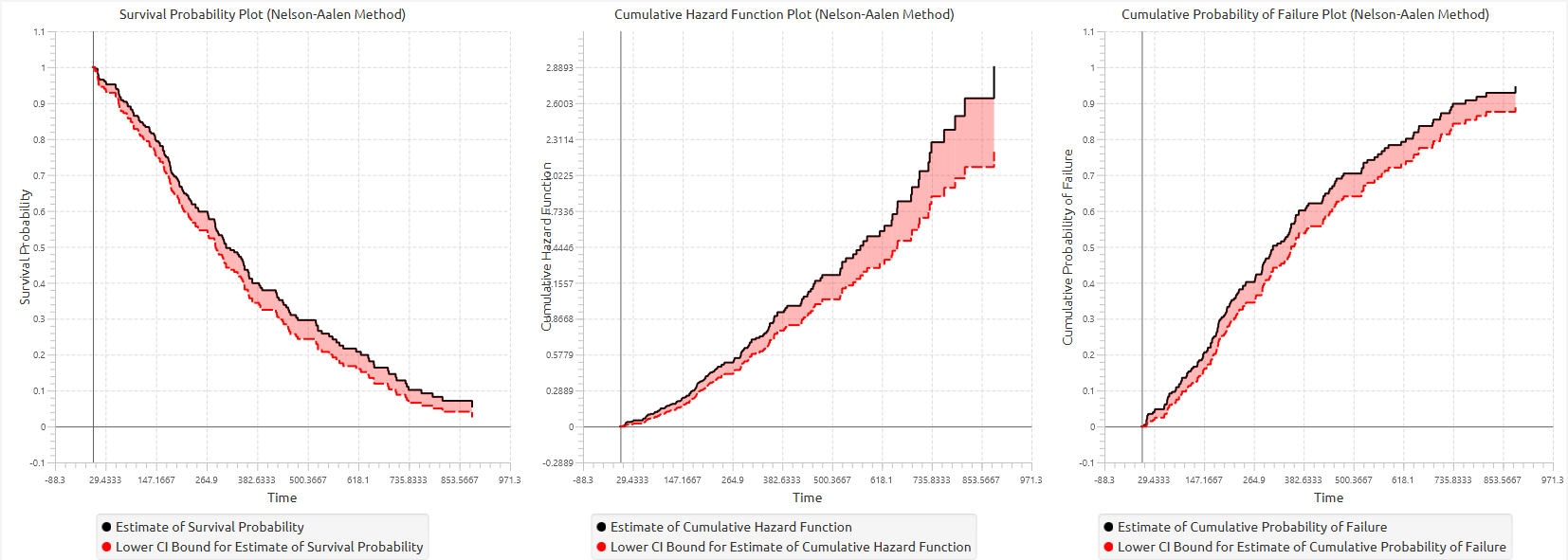
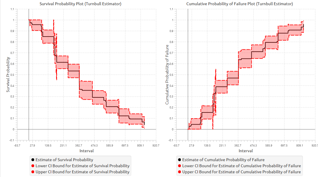
The results are typically visualized using stepwise plots of the survival function and cumulative probability of failure, providing a graphical representation of the distribution of event times under interval censoring.
Use the Turnbull Estimator by browsing in the top ribbon:
Statistics \(\rightarrow\) Survival Analysis \(\rightarrow\) Non-Parametric \(\rightarrow\) Turnbull Estimator |
Input
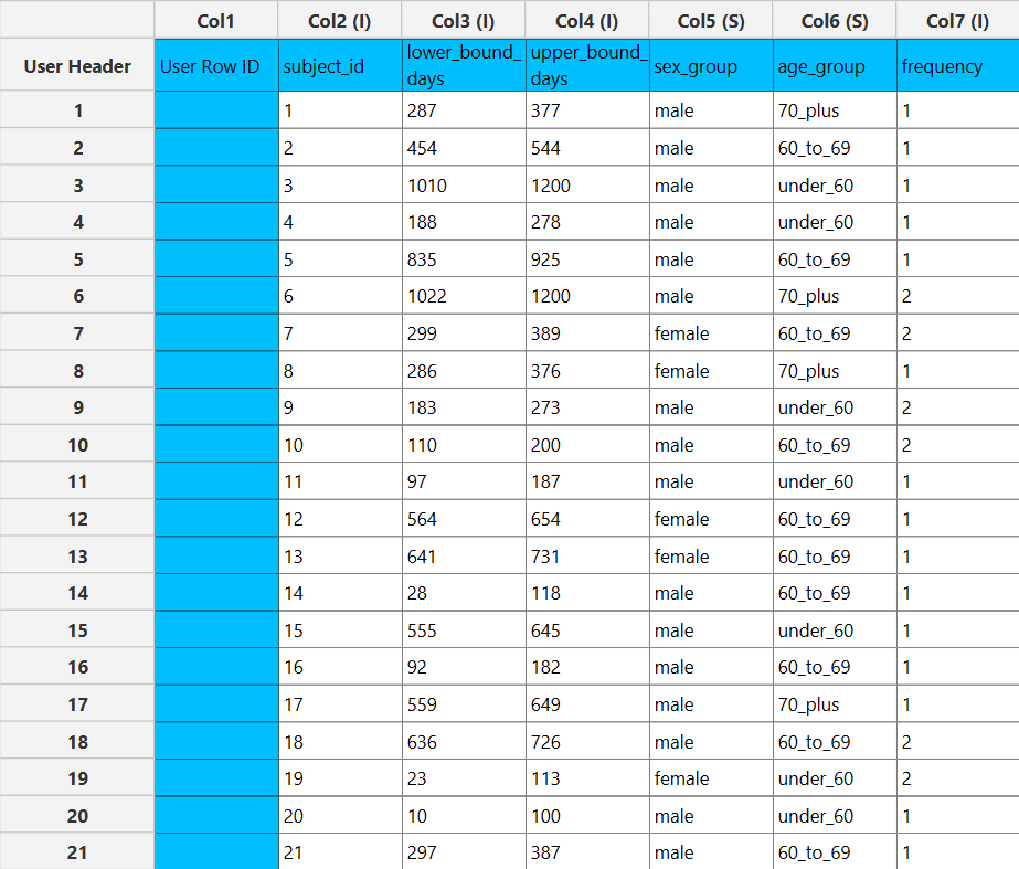
The Turnbull method requires two columns of numerical data to be specified in the input datasheet. The required inputs are a lower bound column and an upper bound column, representing the interval within which the event is known to occur for each observation. These columns must contain non-negative numerical values. Empty cells are allowed in either the lower bound column or the upper bound column to represent left-censored or right-censored observations respectively; however, both values cannot be empty in the same row. In addition, when both bounds are specified, the lower bound must not exceed the upper bound. In addition to the interval bounds, several optional inputs may be provided to extend the functionality of the analysis. A frequency column may also be included, consisting of non-negative numerical values that represent the number of identical observations associated with each row; if this column is not provided, each row is treated as a single observation by default. Furthermore, an event mode column may be defined, which can be either numerical or textual, and is used to distinguish between different types of events depending on the analysis configuration. Finally, a grouping column can be specified as a categorical variable, either numerical or textual, indicating the group membership of each observation. All input columns must be of consistent type and should not contain invalid or missing values, as this may prevent the method from executing correctly.
Configuration
| Interval Start (Lower Bound) | Select the column corresponding to the lower bound of the interval for each subject. This column must be numerical and contain non-negative values. |
| Interval End (Upper Bound) | Select the column corresponding to the upper bound of the interval for each subject. This column must be numerical and contain non-negative values. For each row the upper bound should be larger or equal to the lower bound. |
| Event Mode Column | Within the Configure Event Mode Options window, specify the column containing event mode information. |
| Levels not Considered as Event/Levels Considered as Event | Manually select which levels should be treated as events from the available levels of the Event Mode Column. Use the arrow buttons to move levels between the two lists. Single-arrow buttons move selected levels, while double-arrow buttons move all levels. At least one level must be selected as an event. |
| Clear Event Mode Options | Use this button to clear all selections related to event mode configuration. |
| Use a Frequency Column | Enable this option to include a frequency column in the analysis. |
| Frequency Column | If the Use a Frequency Column option is enabled, select the column containing frequency information for each observation. This column must be numerical and contain non-negative values. |
| Use a Grouping Column | Enable this option to include a grouping column in the analysis, allowing comparison of survival across different groups in the population. |
| Grouping Column | If the Use a Grouping Column option is enabled, select the column containing grouping information for each observation. This column must be categorical. |
| Confidence Level (%) | Specify the confidence level of the analysis. Values should range from 0 to 100 and correspond to percentages. Default value is set to 95. |
| Confidence Interval Type | Select the type of confidence interval to compute. Available options include: Two-sided, Lower Bound, Upper Bound. |
| Cumulative Probability of Failure Plot | Enable this option to generate a plot of the estimated cumulative probability of failure over time. |
| Max Iterations | Specify the maximum number of iterations for the EM algorithm. The default value is 1000. |
| Convergence Tolerance | Specify the convergence tolerance for the EM algorithm. The default value is \(10^{-7}\) |
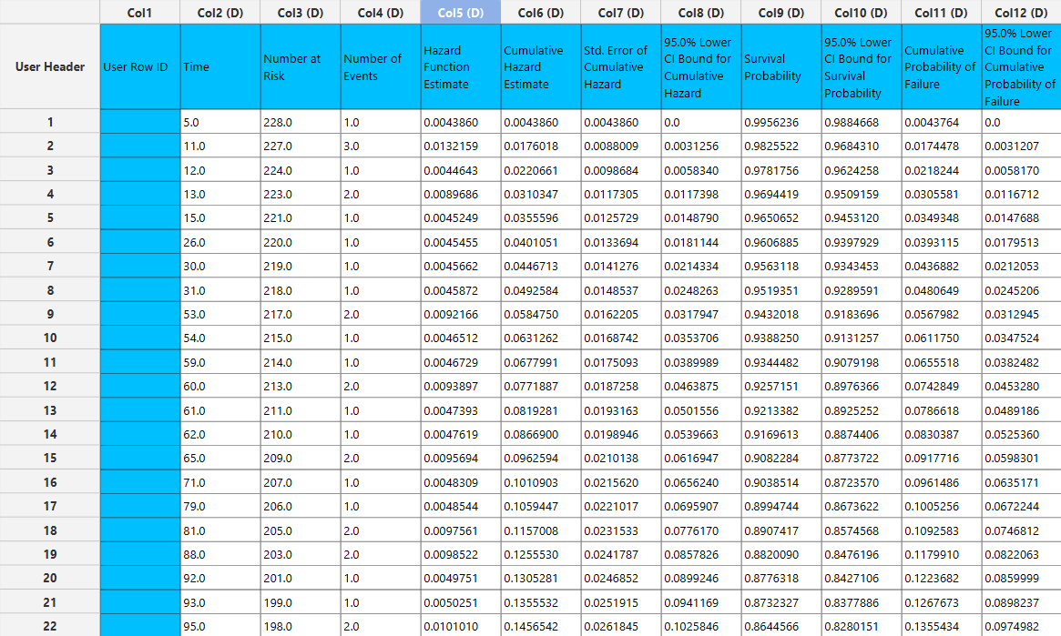
Output
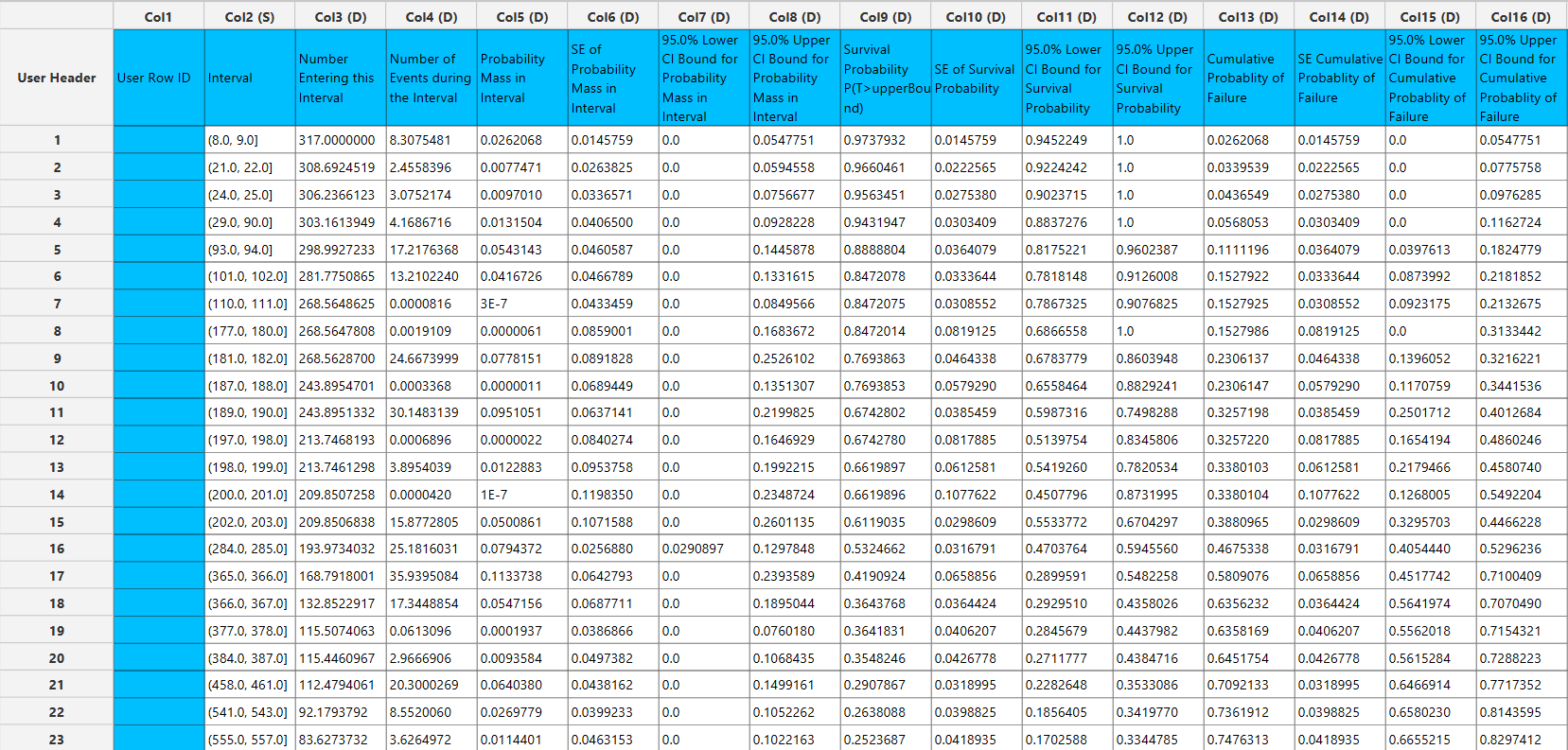
The output spreadsheet contains a table summarizing the survival analysis results at each interval. This includes the number entering the interval, the number of events during the interval, the estimated probability mass for the interval, the estimated survival probability and the cumulative probability of failure, along with their standard errors, and the corresponding confidence interval bounds at the selected confidence level. If a grouping column is specified, the spreadsheet first presents the overall results for the full sample, followed by separate tables for each group.
In addition, a pop-up window displays the Kaplan–Meier survival curve, showing the stepwise estimate of survival probability over time along with the associated confidence interval bounds. When grouping is enabled, the plot includes the overall survival curve as well as separate curves with confidence bounds for each group. Similarly, if selected, cumulative probability of failure plot is generated and displays both the overall estimates and the corresponding group-specific curves.
Example
Input
In the input datasheet the requirement is to specify at least two numerical column and insert the appropriate data, as shown below.
Configuration
- Select
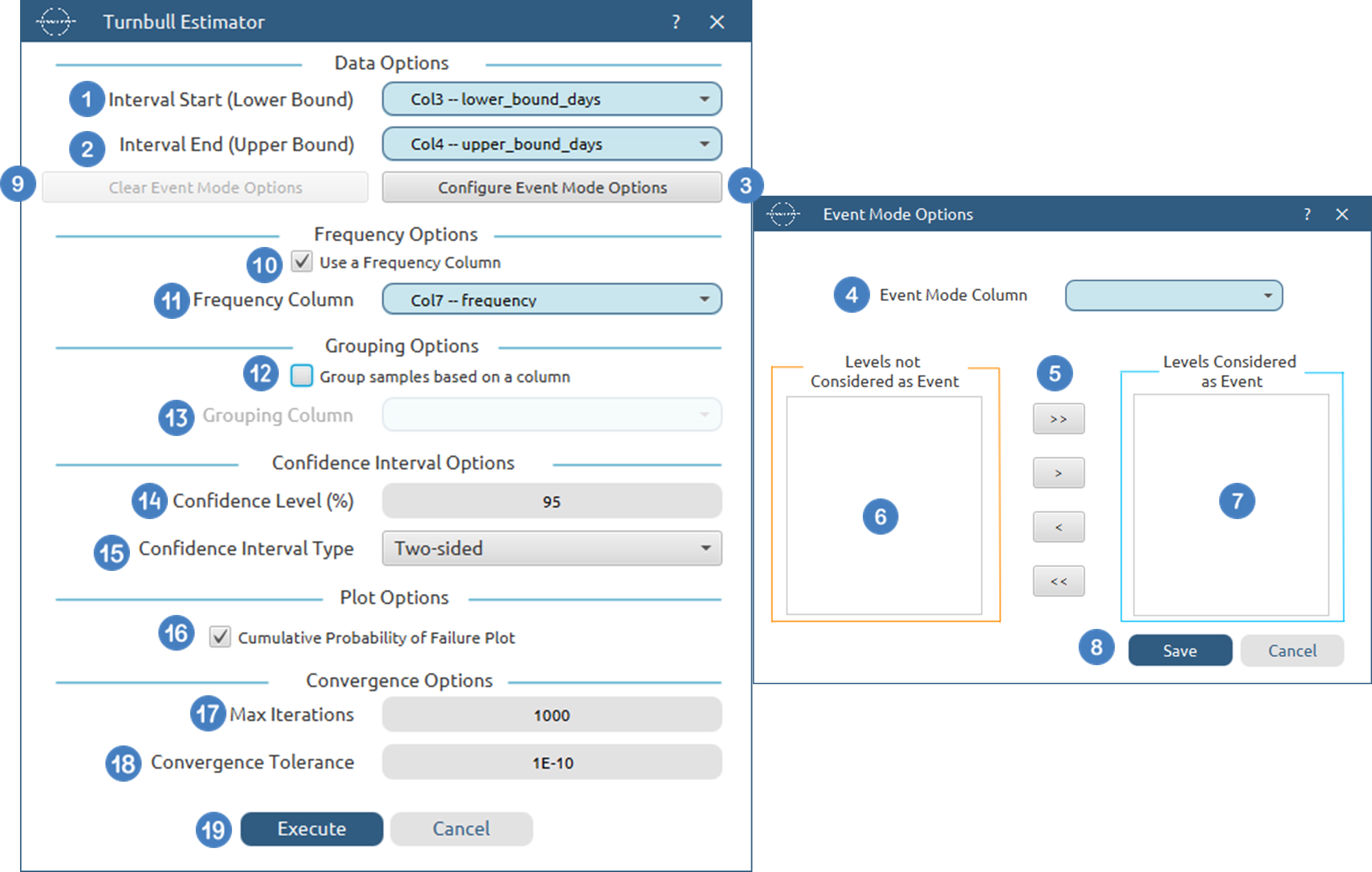
Statistics→Survival Analysis→Non-Parametric→Turnbull Estimator. - Select the column that contains the
Interval Start (Lower Bound)[1] andd the column that contains theInterval End (Upper Bound)[2] for each subject. These columns should contain non-negative numeric values. - Optionally click on the
Configure Event Mode Options[3] button to select anEvent Mode Column[4] and use the arrow buttons [5] to select the levels that should be accounted for in the analysis by moving them between theLevels not Considered as Event[6] andLevels Considered as Event[7] lists.SaveorCancelany changes made using the appropriate buttons [8]. - Once you have configured some Event Mode Options you can optionally use the
Clear Event Mode Options[9] button to erase any selections made. - Select/tick to
Use a Frequency Column[10]. - If the
Use a Frequency Columnoption is selected, specify aFrequency Column[11]. This column should contain non-negative numeric values. - Select/tick to
Use a Grouping Column[12]. - If the
Use a Grouping Columnoption is selected, specify aGrouping Column[13]. This column should be categorical, either textual or numerical. - Specify the
Confidence Level(%) [14] for Confidence Intervals and the desiredConfidence Interval Type[15]. - Optionally select/tick to calculate and present the
Cumulative Probability of Failure Plot[16]. - Specify the
Max Iterations[17] of the iterative algorithm to perform and theConvergence Tolerance[18]. - Click on the
Executebutton [19] to perform the Turnbull Estimator.
Output
The tables summarizing the survival analysis results for the non grouped dataset and each grouping level are shown in the output spreadsheet. In addition, a pop-up window displays the Turnbull survival curve and, if selected, the cumulative probability of failure plot.
Survival Curve Comparison Tests
Survival curve comparison tests are non-parametric statistical procedures used to assess whether two or more groups share the same underlying hazard function over time. These tests are based on weighted comparisons between the observed number of events in each group and the number expected under the null hypothesis of equal hazard rates.
The general null hypothesis tested is
against the alternative that at least one group differs at some point in time.
These methods operate on the ordered distinct event times in the pooled sample. At each event time \(t_i\), the following quantities are defined:
- \(d_{ij}\): number of events in group j at time \(t_i\).
- \(Y_{ij}\): number of individuals at risk in group j just prior to \(t_i\).
- \(d_i = \sum_{j=1}^Kd_{ij}\): total number of events at time \(t_i\).
- \(Y_i = \sum_{j=1}^KY_{ij}\): total number at risk at time \(t_i\).
Observations may contribute with frequency weights if a frequency column is provided. Censoring is handled in the same manner as in other non-parametric methods: censored observations contribute to the risk set up to their censoring time and are removed thereafter.
Test Statistic
All available tests belong to the class of weighted log-rank tests. For each group j, a test statistic is constructed as
where:
- \(W(t_i)\) is a non-negative weight function
- \(d_{ij}\) the observed number of events
- \(Y_{ij} \frac{d_i}{Y_i}\) is the expected number of events under \(H_0\).
Thus, each test compares the observed and expected number of events at each time point, with differences weighted according to \(W(t_i)\)
Variance and Covariance
The variance of the statistic for group j is estimated as
and the covariance between groups j and g is
These expressions account for ties through the factor \(\frac{Y_i-d_i}{Y_i-1}\).
Overall Test Statistic
Since the group-specific statistics are linearly dependent, the overall test is based on K−1 independent components. The test statistic is
which asymptotically follows a chi-square distribution with K−1 degrees of freedom.
Weight Functions and Available Tests
The different tests arise from different choices of the weight function \(W(t_i)\), which determine how deviations between observed and expected events are emphasized over time.
Log-Rank Test
The log-rank test assigns equal weight to all event times. It is most powerful when the hazard functions of the groups are proportional over time and differences are consistent throughout the study period.
Log-Rank Test
The log-rank test assigns equal weight to all event times. It is most powerful when the hazard functions of the groups are proportional over time and differences are consistent throughout the study period.
Wilcoxon (Breslow) Test
This test gives more weight to early event times, where the number at risk is largest. As a result, it is more sensitive to differences that occur early in time.
Peto–Peto Test
The Peto–Peto test uses a modified estimate of the pooled survival function
and defines the weight function as
This approach retains the early-time emphasis of the Wilcoxon test but adjusts for censoring, making it more robust when censoring patterns differ between groups.
Tarone–Ware Test
The Tarone–Ware test provides an intermediate weighting scheme between the log-rank and Wilcoxon tests. It balances sensitivity across early and later time points, giving moderate emphasis to the middle range of the follow-up period.
Fleming–Harrington Test
The Fleming–Harrington class of tests uses a flexible weight function based on the pooled Kaplan–Meier survival estimate \(\hat{S}(t)\)
The parameters p and q control the emphasis:
- \(p>0\) increases sensitivity to early differences
- \(q>0\) increases sensitivity to late differences
- \((p,q)=(0,0)\) reduces to the log-rank test
This class provides a flexible framework for targeting specific types of departures from the null hypothesis.
All tests assess whether the observed number of events in each group deviates significantly from what would be expected under equal hazard rates. The choice of weight function determines the sensitivity of the test to differences occurring at different parts of the time axis:
- Early differences → Wilcoxon, Peto–Peto, Fleming–Harrington with p>0
- Late differences → Fleming–Harrington with q>0
- Consistent differences → Log-rank
- Balanced sensitivity → Tarone–Ware
Use the Survival Curve Comparison Tests by browsing in the top ribbon:
Statistics \(\rightarrow\) Survival Analysis \(\rightarrow\) Non-Parametric \(\rightarrow\) Survival Curve Comparison Tests |
Input
The Survival Curve Comparison Tests require at least two columns, one of numerical data and one with categorical data to be specified in the input datasheet. The required input is a time variable column containing non-negative numerical values, representing the observed time-to-event or time-to-censoring for each subject and a grouping column indicating the group membership of each observation. In addition to the time variable, several optional inputs may be provided to extend the functionality of the analysis. A censoring column may be specified as a categorical variable, either numerical or textual, indicating whether each observation corresponds to an event or a censored case. A frequency column may also be included, consisting of non-negative numerical values that represent the number of identical observations associated with each row; if this column is not provided, each row is treated as a single observation by default. Furthermore, an event mode column may be defined, which can be either numerical or textual, and is used to distinguish between different types of events depending on the analysis configuration. All input columns must be of consistent type and should not contain invalid or missing values, as this may prevent the method from executing correctly.
Configuration
| Time Column | Select the column corresponding to the observed time-to-event or time-to-censoring for each subject. This column must be numerical and contain non-negative values. |
| Configure Event Mode Options | Use this button to open the Configure Event Mode Options window |
| Event Mode Column | Within the Configure Event Mode Options window, specify the column containing event mode information. |
| Levels not Considered as Event/Levels Considered as Event | Manually select which levels should be treated as events from the available levels of the Event Mode Column. Use the arrow buttons to move levels between the two lists. Single-arrow buttons move selected levels, while double-arrow buttons move all levels. At least one level must be selected as an event. |
| Clear Event Mode Options | Use this button to clear all selections related to event mode configuration. |
| Use a Frequency Column | Enable this option to include a frequency column in the analysis. |
| Frequency Column | If the Use a Frequency Column option is enabled, select the column containing frequency information for each observation. This column must be numerical and contain non-negative values. |
| Use a Censoring Column | Enable this option to include a censoring column in the analysis. |
| Censoring Column | If the Use a Censoring Column option is enabled, select the column containing censoring information for each observation. This column must be categorical and may be either numerical or textual. |
| Censoring Indicator Value | If a censoring column is used, specify which of its two levels represents a censored observation. |
| Censor times at or above a value | Enable this option to treat all time values greater than or equal to a specified threshold as censored. |
| Censoring Threshold Value | If the Censor times at or above a value option is enabled, specify the value above or equal to which observations will be treated as censored. |
| Grouping Column | Select the column containing grouping information for each observation. This column must be categorical. At least two distinct groups are required to perform the comparison tests. |
| Log-Rank Test | Enable this option to calculate the Log-Rank test |
| Wilcoxon Test | Enable this option to calculate the Wilcoxon test |
| Peto-Peto Test | Enable this option to calculate the Peto-Peto test. |
| Tarone-Ware Test | Enable this option to calculate the Tarone-Ware test |
| Fleming-Harrington Test | Enable this option to calculate the Fleming-Harrington test. |
| Fleming-Harrington Parameters | If the Fleming-Harrington Test option is enabled, specify the values for the two parameters (p, q) of the test. |
Output
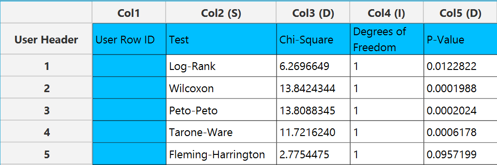
The output spreadsheet contains a table summarizing the non-parametric comparison tests that were selected. For each selected test this included the name of the test, the test statistic, the degrees of freedom and the calculated p-value of the test.
Example
Input
In the input datasheet the requirement is to specify at least one numerical column and insert the appropriate data, as shown below.
Configuration
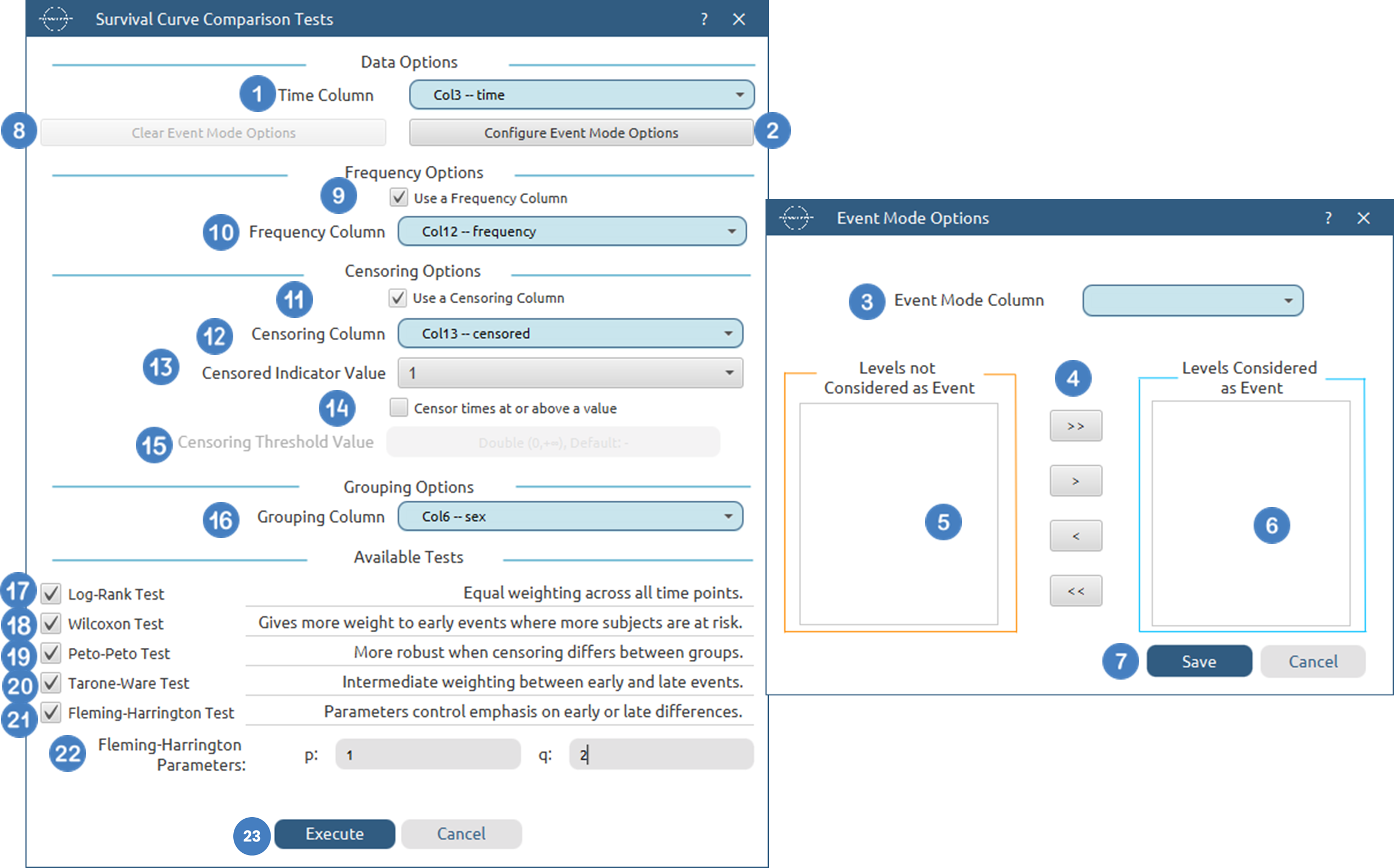
- Select
Statistics→Survival Analysis→Non-Parametric→Survival Curve Comparison Tests. - Select the
Time Column[1]. This column should contain non-negative numeric values. - Optionally click on the
Configure Event Mode Options[2] button to select anEvent Mode Column[3] and use the arrow buttons [4] to select the levels that should be accounted for in the analysis by moving them between theLevels not Considered as Event[5] andLevels Considered as Event[6] lists.SaveorCancelany changes made using the appropriate buttons [7]. - Once you have configured some Event Mode Options you can optionally use the
Clear Event Mode Options[8] button to erase any selections made. - Select/tick to
Use a Frequency Column[9]. - If the
Use a Frequency Columnoption is selected, specify aFrequency Column[10]. This column should contain non-negative numeric values. - Select/tick to
Use a Censoring Column[11]. - If the
Use a Censoring Columnoption is selected, specify aCensoring Column[12] and the value of this column that should be theCensored Indicator Value[13]. - Select/tick to
Censor times at or above a value[14]. - If the ``Censor times at or above a value
option is selected, specify aCensoring Thresholdd Value`[15] above which events are considered censored. - Specify a
Grouping Column[16]. This column should be categorical, either textual or numerical. - Select/tick to perform a
Log-Rank Test[17]. - Select/tick to perform a
Wilcoxon Test[18]. - Select/tick to perform a
Peto-Peto Test[19]. - Select/tick to perform a
Tarone-Ware Test[20]. - Select/tick to perform a
Fleming-Harrington Test[21]. If you select to perform such test, specify theFleming-Harrington Parameters[22] :pandq. - Click on the
Executebutton [23] to perform Survival Curve Comparison Tests.
Output
The tables summarizing the survival curve comparison tests results is shown in the output spreadsheet.
Semi-Parametric Methods
Semi-parametric methods in survival analysis combine elements of both parametric and non-parametric approaches. They avoid making strict assumptions about the baseline distribution of survival times, while still incorporating a structured model to assess the effect of covariates on the hazard function. This balance provides flexibility alongside inferential power, making these methods central to modern survival analysis.
The most prominent semi-parametric framework is the Cox Proportional Hazards Model, which models the hazard function as a product of an unspecified baseline hazard and a parametric component driven by covariates. This allows estimation of relative risk effects without requiring explicit specification of the underlying time-to-event distribution.
Two key variants of this method are included:
- Fixed Covariates Model: Assumes that covariates remain constant over time for each subject. The model evaluates how these baseline characteristics proportionally affect the hazard.
- Time-Dependent Covariates Model: Allows covariates to change over time, enabling more realistic modeling of dynamic systems where subject characteristics evolve during the observation period.
Semi-parametric methods are primarily used to:
- Estimate the effect of covariates on the hazard function without specifying the baseline hazard
- Handle censored data naturally within the partial likelihood framework
- Model relative risks through hazard ratios, enabling interpretation of covariate impact
- Incorporate both static and time-dependent covariates for more flexible modeling
- Provide a bridge between exploratory non-parametric methods and fully specified parametric models
These methods are typically applied after initial exploratory analysis, offering a robust and interpretable way to quantify relationships between predictors and survival outcomes without imposing restrictive distributional assumptions.
An important aspect of model specification in Cox regression is the handling of tied event times and the choice of variance–covariance estimation method.
When multiple events occur at the same observed time, a tie-handling method must be specified. Common approaches include the Breslow and Efron methods. The Breslow method provides a simpler approximation and is computationally efficient, but may be less accurate when there are many tied events. The Efron method offers a more refined approximation by accounting for the ordering of tied events within a risk set and generally provides better accuracy in moderate to large samples. However, it requires that frequency values (if used) are integers, as it relies on discrete event counts.
The variance–covariance type determines how uncertainty in the estimated coefficients is quantified. The model-based (naïve) variance estimator assumes that the model is correctly specified and that observations are independent, providing efficient estimates under these assumptions. In contrast, the robust (sandwich) variance estimator relaxes these assumptions and provides standard errors that are consistent even in the presence of model misspecification or correlated observations (e.g., clustered or repeated measures data). When the robust estimator is used, certain likelihood-based inference procedures—such as likelihood ratio tests and related ANOVA components—are not valid and therefore cannot be estimated, while Wald and robust score tests remain applicable.
Cox Proportional Hazards with Fixed Covariates
The Cox Proportional Hazards Model with fixed covariates is a semi-parametric survival regression method used to evaluate how predictor variables affect the risk of an event occurring over time. The model does not require a specific distribution for survival times. Instead, it estimates covariate effects through the partial likelihood while leaving the baseline hazard function unspecified.
In this model, each subject has one fixed set of predictor values throughout the observation period. These predictors may include continuous covariates, categorical factors, interaction terms, or custom formula terms. The model estimates regression coefficients that describe how each predictor changes the hazard relative to a baseline risk.
The hazard function is modeled as:
where \(h_0(t)\) is the unspecified baseline hazard, x is the vector of fixed covariates, and \(\beta\) is the vector of estimated coefficients.
This method supports:
- Right-censored survival data
- Optional frequency weights
- Optional event-mode filtering
- Optional administrative censoring at a specified censoring value
- Optional entry times for delayed entry / left truncation
- Optional stratification of the baseline hazard
- Continuous covariates and categorical factors
- Custom model formulas, main-effects models, and full factorial models
- Model-based or robust variance estimation
- Cluster-adjusted robust standard errors
- Multiple tie-handling methods, including Breslow
- Predicted survival curves for user-specified covariate patterns
The model output includes coefficient estimates, standard errors, confidence intervals, Wald statistics, degrees of freedom, and p-values for each fitted parameter. Coefficients are usually interpreted through hazard ratios, where positive coefficients increase the hazard and negative coefficients decrease the hazard.
The method also provides model-level summaries, including the partial log-likelihood, pseudo \(R_2\), AIC, AICc, BIC, and CAIC. Goodness-of-fit tests may include Wald, likelihood ratio, and score tests when model-based variance estimation is used. When robust variance estimation is selected, Wald and robust score tests are reported.
Stratification may be used when different groups are expected to have different baseline hazard functions but the same covariate effects. In that case, the baseline cumulative hazard is estimated separately for each stratum, while the regression coefficients remain common across strata.
This model is useful when the primary goal is to quantify the association between predictors and survival outcomes while avoiding strong assumptions about the shape of the underlying survival distribution.
Use the Cox Proportional Hazards Model with Fixed Covariates by browsing in the top ribbon:
Statistics \(\rightarrow\) Survival Analysis \(\rightarrow\) Semi-Parametric \(\rightarrow\) Cox Proportional Hazards Model with Fixed Covariates |
Input
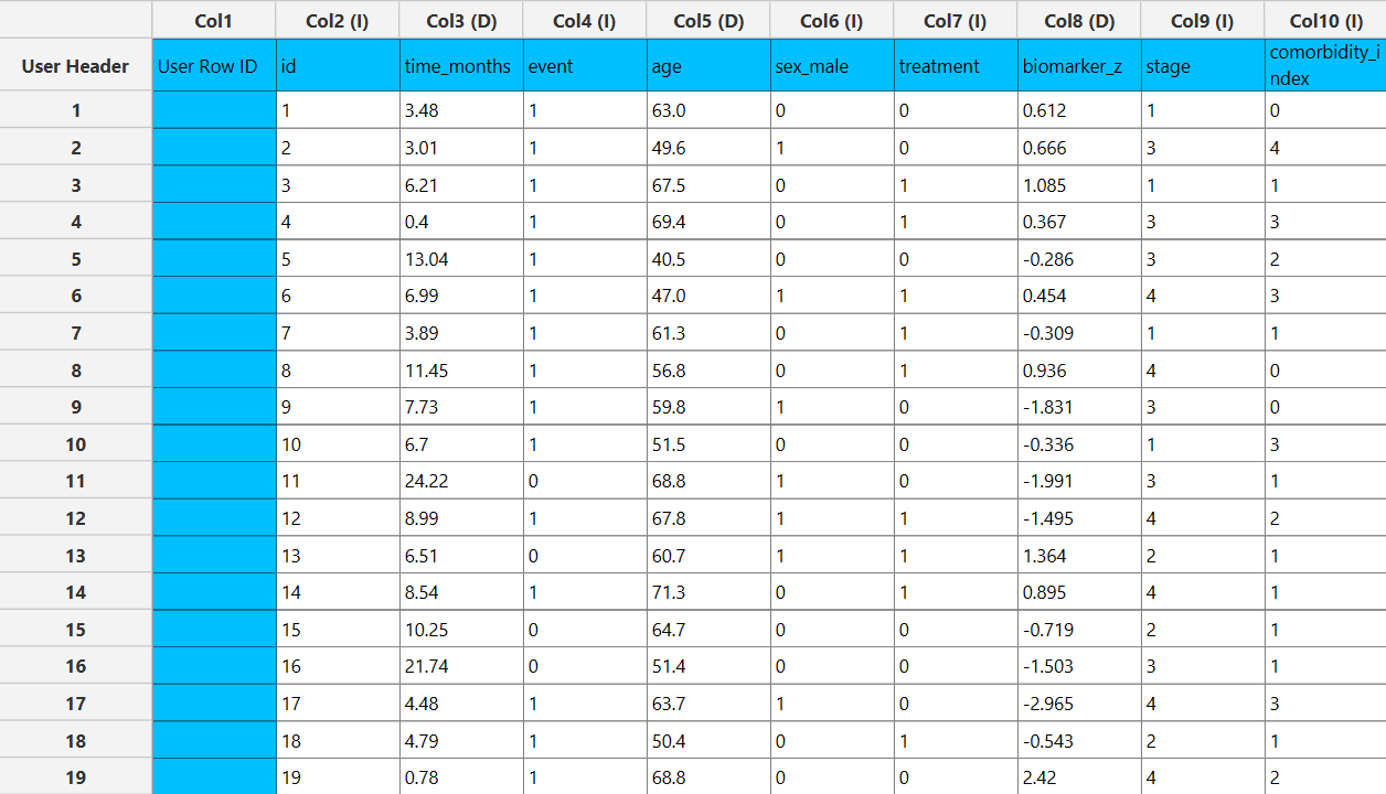
The Cox Proportional Hazards Model with Fixed Covariates requires at least two columns to be specified in the input datasheet: one numerical time column and at least one predictor variable. The time column must contain non-negative numerical values representing the observed time-to-event or time-to-censoring for each subject. Predictor variables may be specified either as categorical factors or numerical covariates and are used to model their effect on the hazard of the event occurring.
In addition to the time variable and predictor variables, several optional inputs may be provided to extend the analysis. A censoring column may be specified as a numerical or textual variable indicating whether each observation corresponds to an event or a censored case. A frequency column may be included, consisting of non-negative numerical values that represent the number of identical observations associated with each row; if this column is not provided, each row is treated as a single observation by default. An event mode column may also be defined, using numerical or textual values to distinguish between different event types and determine which observations should be included in the analysis. An entry time column may be provided to account for delayed entry or left-truncated observations, where subjects enter the risk set after time zero.
The method may also include a stratification column, which defines groups with separate baseline hazard functions while keeping the same covariate effects across strata. If robust variance estimation is selected, a cluster ID column may be specified to compute cluster-adjusted standard errors.
Categorical factors may require reference levels, while numerical covariates are entered directly into the model. The selected predictors may be combined using a custom model formula, main-effects model, or full factorial model. All input columns must be of consistent type and should not contain invalid or missing values, as this may prevent the method from executing correctly.
Configuration
| Time Column | Select the column corresponding to the observed time-to-event or time-to-censoring for each subject. This column must be numerical and contain non-negative values. |
| Configure Response Options | Use this button to open the Configure Response Options window to configure Event Mode, Frequency, Censoring and Entry Time Options More on Response Options |
| Clear Response Options | Use this button to clear all selections related to the response configuration. |
| Stratify baseline hazard by a column | Enable this option to allow different baseline hazard functions across groups defined by a stratification column, while keeping the same covariate effects across all strata. |
| Stratification Column | Select the categorical column used to define strata. Each level will have its own baseline hazard function. This option is only available when stratification is enabled. |
| Confidence Level (%) | Specify the confidence level of the analysis. Values should range from 0 to 100 and correspond to percentages. Default value is set to 95. |
| Confidence Interval Type | Select the type of confidence interval to compute. Available options include: Two-sided, Lower Bound, Upper Bound. |
| Tie Handling Method | Specify the method used to handle tied event times. Available options include methods such as Breslow and Efron. The Efron method can only be used when frequency values are integers, as it relies on discrete event counts. |
| Variance/Covariance Type | Select the method used to estimate the variance-covariance matrix of the coefficients. Options include Model-based and Robust. The robust option provides sandwich (cluster-adjusted) standard errors that are less sensitive to model misspecification. |
| Cluster ID Column | Select the column identifying clusters of observations. This option is optional and is only available when the robust variance option is selected. It is used to compute cluster-adjusted standard errors. |
| Max Iterations | Specify the maximum number of iterations allowed for the optimization algorithm (Newton-Raphson). Higher values may be required for complex models but will increase computation time. Default value is set to 25. |
| Minimum Change in Estimates | Define the convergence threshold for the optimization algorithm. The algorithm stops when the change in parameter estimates between iterations falls below this value. Default value is set to 1e-6. |
| Factors/ Covariates / Excluded columns | Select manually the columns that correspond to factors and the columns that correspond to covariates through the dialog window: Use the buttons to move columns between the Factors and Covariates list and Excluded Columns list. Single-arrow buttons will move all selected columns and double-arrow buttons will move all columns. At least one covariate column should be specified. |
| Specify Reference Levels | Specify the reference level for each of the categorical factors specified. The default option for each factor is its last level. |
| Formula Type | These options refer to the terms that will be included in the model. The Custom option allows the user to input a formula defining the exact terms to be included. The Main Effects option allows the analysis of a model that only includes all main effects and finally, the Full Factorial option includes both all main effects and all possible interaction terms to build a full model. |
| Specify Custom Model Formula | Specify the model formula used for the analysis if the Custom option is selected. The formula is created in the Custom Formula Creation dialog window by selecting factors and covariates and adding interaction terms up to the required order. Main effects of the included columns are always part of the model and cannot be excluded. |
| Use default prefictor variable values for plots | When enabled, predicted survival curves are generated using default values for predictors. These defaults are the reference levels for categorical factors and the midpoints of the observed ranges for numerical covariates. |
| Specify Predictor Variable Values for the plot | Define custom values for predictors to generate predicted survival curves. The user may specify up to 10 different sets of predictor values, and a separate survival curve will be produced for each set. |
Output
The output of the Cox Proportional Hazards Model with Fixed Covariates is presented in a structured spreadsheet containing multiple tables that summarize the fitted model, statistical inference, and overall model performance.
The main output includes a Parameter Estimates table, which reports the estimated regression coefficients for each covariate, along with their corresponding standard errors, confidence interval bounds at the selected confidence level, test statistics, degrees of freedom, and p-values.
A Goodness-of-Fit table is also provided, summarizing key model diagnostics including the partial log-likelihood, pseudo \(R^2\), Akaike Information Criterion (AIC), finite-sample corrected AIC (AICc), Bayesian Information Criterion (BIC), and Consistent AIC (CAIC). These measures allow for assessment of model fit and comparison between competing models.
In addition, a Goodness-of-Fit Tests table is included, presenting global hypothesis tests for the model. When model-based variance estimation is selected, this table includes Wald, likelihood ratio, and score tests, each with their associated degrees of freedom, test statistics, and p-values. If the robust variance estimator is selected, the likelihood ratio test cannot be estimated.
An ANOVA table is also generated, providing term-wise inference for each predictor (and interaction terms, if specified). This table includes Wald, likelihood ratio, and score test statistics and p-values for each model term when model-based variance estimation is used. If the robust variance estimator is selected, the likelihood ratio and score ANOVA tests cannot be estimated, and only Wald-based results are reported.
In addition to the tabular output, a pop-up window displays the predicted survival probability curves based on the fitted model. These curves are computed using the estimated coefficients and the baseline cumulative hazard function. Confidence interval bounds are displayed according to the selected confidence interval type. When multiple sets of predictor values are specified, a separate survival curve (with confidence bounds) is plotted for each set, allowing direct comparison of survival profiles under different covariate configurations.
Example
Input
In the input datasheet the requirement is to specify at least two columns, from which at least one should be numerical and insert the appropriate data, as shown below.
Configuration
- Select
Statistics→Survival Analysis→Semi-Parametric→Cox Proportional Hazards with Fixed Covariates. - Select the
Time Column[1]. This column should contain non-negative numeric values. - Optionally click on the
Configure Response Options[2] button to specify various response options including Event Mode, Frequency, Censoring and Entry Time. Within theSurvival Response Optionswindow:- Select/tick to
Use an Event Mode Column[3]. - If the
Use an Event Mode Columnoption is selected, specify anEvent Mode Column[4] and use the arrow buttons [5] to select the levels that should be accounted for in the analysis by moving them between theLevels not Considered as Event[6] andLevels Considered as Event[7] lists. - Select/tick to
Use an Entry Time Column[8]. - If the
Use an Entry Time Columnoption is selected, specify anEntry Time Column[9]. This column should contain non-negative numeric values. - Select/tick to
Use a Frequency Column[10]. - If the
Use a Frequency Columnoption is selected, specify aFrequency Column[11]. This column should contain non-negative numeric values. - Select/tick to
Use a Censoring Column[12]. - If the
Use a Censoring Columnoption is selected, specify aCensoring Column[13] and the value of this column that should be theCensored Indicator Value[14]. - Select/tick to
Censor times at or above a value[15]. - If the ``Censor times at or above a value
option is selected, specify aCensoring Thresholdd Value`[16] above which events are considered censored. SaveorCancelany changes made using the appropriate buttons [17].
- Select/tick to
- Once you have configured some Response Options you can optionally use the
Clear Response Options[18] button to erase any selections made. - Select/tick to
Stratify baseline hazard by a column[19]. - If the
Stratify baseline hazard by a columnoption is selected, specify aStratification Column[20]. This column should be categorical, either textual or numerical. - Specify the
Confidence Level(%) [21] for Confidence Intervals and the desiredConfidence Interval Type[22]. - Select between the two available
Tie handling methods[23]. - Select whether to use a Model-based or a Robust
Variance/Covariance Type[24]. - If the Robust
Variance/Covariance Typeis selected, optionally select aCluster ID Column[25]. - Specify the
Max Iterations[26] of the iterative algorithm to perform and theMinimum Change in Parameter Estimates[27]. - Select the columns by clicking on the arrow buttons [28] and moving columns between the
Excluded Columns[29] andFactors[30] andCovariates[31] lists. - Optionally, specify
Specify Reference Levels[32] for the categorical factors. - Select the prefered
Formula Type[33]. Specify Custom Model Formula[34] for the analysis ifCustomoption is selected. How to specify a custom model formula?- Select/tick to
Use default predictor variable values for plots[35], otherwiseSpecify Predictor Variable Values for the plots[36]. - Click on the
Executebutton [37] to perform the Cox Proportional Hazards Model with Fixed Covariates.
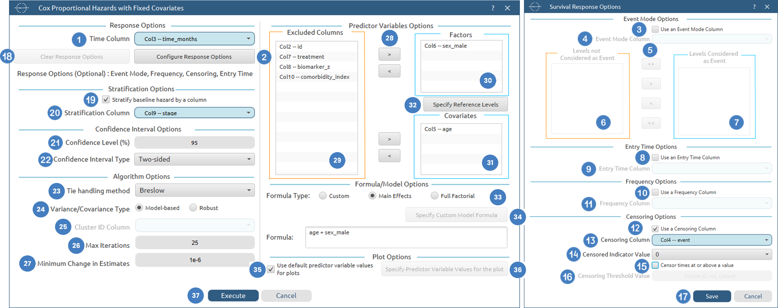
Output
The tables summarizing the survival analysis results for the cox proportional hazards model with fixed covariates are shown in the output spreadsheet. In addition, a pop-up window displays the survival curve for each of the selected sets of covariate settings.
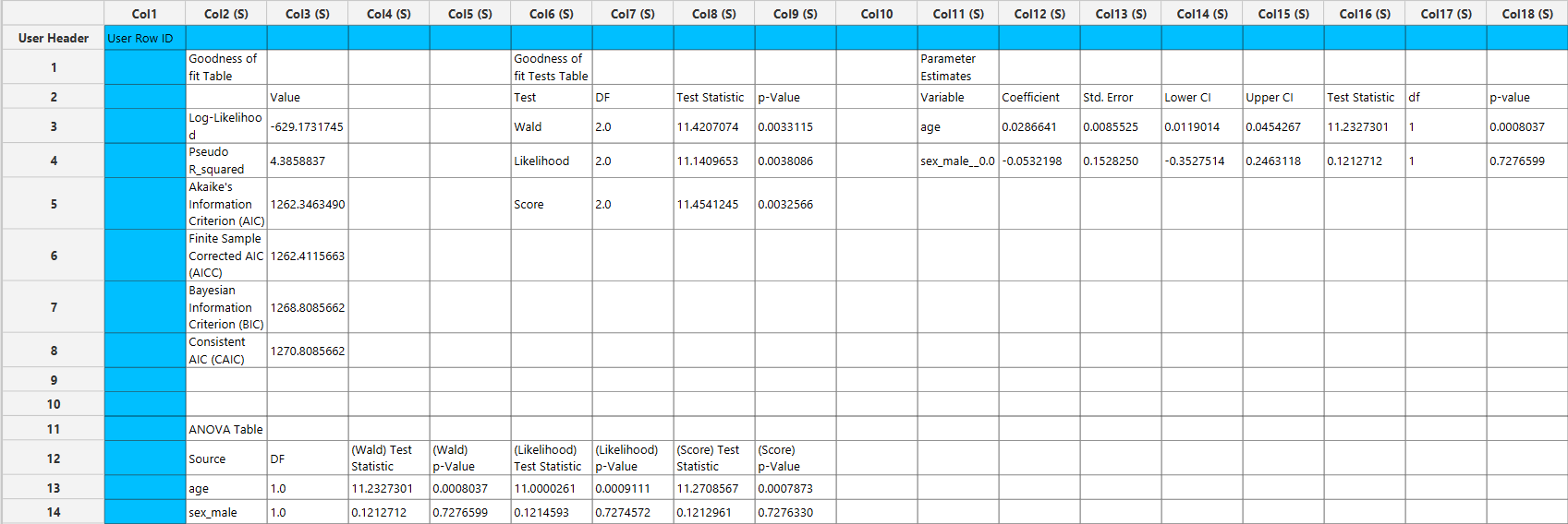
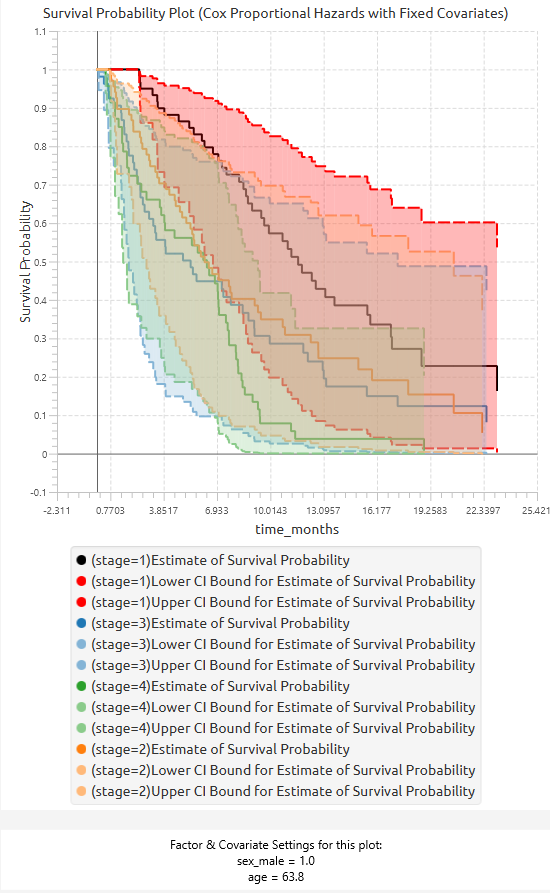
Cox Proportional Hazards with Time-Dependent Covariates
The Cox Proportional Hazards Model with Time-Dependent Covariates is a semi-parametric survival regression method used when predictor values may change over the observation period. Instead of representing each subject with a single row, the data are organized into intervals, where each row describes the covariate values that apply during a specific time interval.
The model does not assume a specific distribution for survival times. It estimates covariate effects through the Cox partial likelihood while leaving the baseline hazard function unspecified. The hazard function is modeled as: The hazard function is modeled as:
where \(h_0(t)\) is the unspecified baseline hazard, \(x(t)\) is the vector of covariates at time t, and \(\beta\) is the vector of estimated coefficients.
This method supports:
- Start–stop interval survival data
- Time-dependent covariates
- Right-censored observations
- Optional subject ID validation
- Optional frequency weights
- Optional event-mode filtering
- Optional stratification of the baseline hazard
- Continuous covariates and categorical factors
- Custom model formulas, main-effects models, and full factorial models
- Model-based or robust variance estimation
- Optional cluster-adjusted robust standard errors
- Multiple tie-handling methods
- Predicted survival curves for user-specified covariate profiles
Each subject may contribute multiple rows, provided that their time intervals do not overlap. If a subject ID column is specified, the method checks that each subject has non-overlapping intervals, no more than one event, and that any event occurs only in the subject’s final interval.
Use the Cox Proportional Hazards Model with Time-Dependent Covariates by browsing in the top ribbon:
Statistics \(\rightarrow\) Survival Analysis \(\rightarrow\) Semi-Parametric \(\rightarrow\) Cox Proportional Hazards Model with Time-Dependent Covariates |
Input
The Cox Proportional Hazards Model with Time-Dependent Covariates requires at least three columns to be specified in the input datasheet: an interval start column, an interval end column, and at least one predictor variable.The Interval Start column represents the lower bound of each observation interval, while the Interval End column represents the upper bound of the interval. These columns must contain non-negative numerical values. Together, they define the time interval during which the covariate values in that row are assumed to apply. Predictor variables may be specified as categorical factors or numerical covariates. Because this method supports time-dependent covariates, the same subject may appear in multiple rows with different predictor values across intervals. Several optional inputs may also be provided. A censoring column may be specified as a binary numerical or textual variable indicating whether each interval ends in an event or censoring. A frequency column may be included to represent the number of identical observations associated with each row; if omitted, each row is treated as a single observation. An event mode column may be used to distinguish between different event types and include only selected event modes in the analysis. A subject ID column may also be specified. When provided, it is used to validate repeated rows belonging to the same subject. The method checks that subject intervals do not overlap, that each subject has at most one event, and that an event does not occur before the subject’s final interval. The method may also include a stratification column, which defines groups with separate baseline hazard functions while keeping the same covariate effects across strata. If robust variance estimation is selected, a cluster ID column may optionally be specified to compute cluster-adjusted standard errors. All input columns must be of consistent type and should not contain invalid or missing values, as this may prevent the method from executing correctly.
Configuration
| Interval Start (Lower Bound) | Select the numerical column containing the lower bound of each observation interval. Values must be non-negative. |
| Interval End (Upper Bound) | Select the numerical column containing the upper bound of each observation interval. Values must be non-negative and should define the end of the interval over which the row’s covariate values apply. |
| Configure Response Options | Use this button to open the Configure Response Options window to configure Event Mode, Frequency, Censoring and Subject ID Options More on Response Options |
| Clear Response Options | Use this button to clear all selections related to the response configuration. |
| Stratify baseline hazard by a column | Enable this option to allow different baseline hazard functions across groups defined by a stratification column, while keeping the same covariate effects across all strata. |
| Stratification Column | Select the categorical column used to define strata. Each level will have its own baseline hazard function. This option is only available when stratification is enabled. |
| Confidence Level (%) | Specify the confidence level of the analysis. Values should range from 0 to 100 and correspond to percentages. Default value is set to 95. |
| Confidence Interval Type | Select the type of confidence interval to compute. Available options include: Two-sided, Lower Bound, Upper Bound. |
| Tie Handling Method | Specify the method used to handle tied event times. Available options include methods such as Breslow and Efron. The Efron method can only be used when frequency values are integers, as it relies on discrete event counts. |
| Variance/Covariance Type | Select the method used to estimate the variance-covariance matrix of the coefficients. Options include Model-based and Robust. The robust option provides sandwich (cluster-adjusted) standard errors that are less sensitive to model misspecification. |
| Cluster ID Column | Select the column identifying clusters of observations. This option is optional and is only available when the robust variance option is selected. It is used to compute cluster-adjusted standard errors. |
| Max Iterations | Specify the maximum number of iterations allowed for the optimization algorithm (Newton-Raphson). Higher values may be required for complex models but will increase computation time. Default value is set to 25. |
| Minimum Change in Estimates | Define the convergence threshold for the optimization algorithm. The algorithm stops when the change in parameter estimates between iterations falls below this value. Default value is set to 1e-6. |
| Factors/ Covariates / Excluded columns | Select manually the columns that correspond to factors and the columns that correspond to covariates through the dialog window: Use the buttons to move columns between the Factors and Covariates list and Excluded Columns list. Single-arrow buttons will move all selected columns and double-arrow buttons will move all columns. At least one covariate column should be specified. |
| Specify Reference Levels | Specify the reference level for each of the categorical factors specified. The default option for each factor is its last level. |
| Formula Type | These options refer to the terms that will be included in the model. The Custom option allows the user to input a formula defining the exact terms to be included. The Main Effects option allows the analysis of a model that only includes all main effects and finally, the Full Factorial option includes both all main effects and all possible interaction terms to build a full model. |
| Specify Custom Model Formula | Specify the model formula used for the analysis if the Custom option is selected. The formula is created in the Custom Formula Creation dialog window by selecting factors and covariates and adding interaction terms up to the required order. Main effects of the included columns are always part of the model and cannot be excluded. |
| Use default prefictor variable values for plots | When enabled, predicted survival curves are generated using default values for predictors. These defaults are the reference levels for categorical factors and the midpoints of the observed ranges for numerical covariates. |
| Specify Predictor Variable Values for the plot | Define custom values for predictors to generate predicted survival curves. The user may specify up to 10 different sets of predictor values, and a separate survival curve will be produced for each set. |
Output
The output of the Cox Proportional Hazards Model with Time-Dependent Covariates is presented in a structured spreadsheet containing multiple tables that summarize the fitted model, statistical inference, and overall model performance.
The main output includes a Parameter Estimates table, which reports the estimated regression coefficients for each covariate, along with their corresponding standard errors, confidence interval bounds at the selected confidence level, test statistics, degrees of freedom, and p-values.
A Goodness-of-Fit table is also provided, summarizing key model diagnostics including the partial log-likelihood, pseudo \(R^2\), Akaike Information Criterion (AIC), finite-sample corrected AIC (AICc), Bayesian Information Criterion (BIC), and Consistent AIC (CAIC). These measures allow for assessment of model fit and comparison between competing models.
In addition, a Goodness-of-Fit Tests table is included, presenting global hypothesis tests for the model. When model-based variance estimation is selected, this table includes Wald, likelihood ratio, and score tests, each with their associated degrees of freedom, test statistics, and p-values. If the robust variance estimator is selected, the likelihood ratio test cannot be estimated.
An ANOVA table is also generated, providing term-wise inference for each predictor (and interaction terms, if specified). This table includes Wald, likelihood ratio, and score test statistics and p-values for each model term when model-based variance estimation is used. If the robust variance estimator is selected, the likelihood ratio and score ANOVA tests cannot be estimated, and only Wald-based results are reported.
In addition to the tabular output, a pop-up window displays the predicted survival probability curves based on the fitted model. These curves are computed using the estimated coefficients and the baseline cumulative hazard function. Confidence interval bounds are displayed according to the selected confidence interval type. When multiple sets of predictor values are specified, a separate survival curve (with confidence bounds) is plotted for each set, allowing direct comparison of survival profiles under different covariate configurations.
Example
Input
In the input datasheet the requirement is to specify at least three columns, from which at least two should be numerical and insert the appropriate data, as shown below.

Configuration
- Select
Statistics→Survival Analysis→Semi-Parametric→Cox Proportional Hazards with Time-Dependent Covariates. - Select the column that contains the
Interval Start (Lower Bound)[1] andd the column that contains theInterval End (Upper Bound)[2] for each subject. These columns should contain non-negative numeric values. - Optionally click on the
Configure Response Options[3] button to specify various response options including Event Mode, Frequency, Censoring and Subject ID. Within theSurvival Response Optionswindow:- Select/tick to
Use an Event Mode Column[4]. - If the
Use an Event Mode Columnoption is selected, specify anEvent Mode Column[5] and use the arrow buttons [6] to select the levels that should be accounted for in the analysis by moving them between theLevels not Considered as Event[7] andLevels Considered as Event[8] lists. - Select/tick to
Use a Subject Column[9]. - If the
Use a Subject Columnoption is selected, specify aSubject Column[10]. This column should contain non-negative numeric values. - Select/tick to
Use a Frequency Column[11]. - If the
Use a Frequency Columnoption is selected, specify aFrequency Column[12]. This column should contain non-negative numeric values. - Select/tick to
Use a Censoring Column[13]. - If the
Use a Censoring Columnoption is selected, specify aCensoring Column[14] and the value of this column that should be theCensored Indicator Value[15]. SaveorCancelany changes made using the appropriate buttons [16].
- Select/tick to
- Once you have configured some Response Options you can optionally use the
Clear Response Options[17] button to erase any selections made. - Select/tick to
Stratify baseline hazard by a column[18]. - If the
Stratify baseline hazard by a columnoption is selected, specify aStratification Column[19]. This column should be categorical, either textual or numerical. - Specify the
Confidence Level(%) [20] for Confidence Intervals and the desiredConfidence Interval Type[21]. - Select between the two available
Tie handling methods[22]. - Select whether to use a Model-based or a Robust
Variance/Covariance Type[23]. - If the Robust
Variance/Covariance Typeis selected, optionally select aCluster ID Column[24]. - Specify the
Max Iterations[25] of the iterative algorithm to perform and theMinimum Change in Parameter Estimates[26]. - Select the columns by clicking on the arrow buttons [27] and moving columns between the
Excluded Columns[28] andFactors[29] andCovariates[30] lists. - Optionally, specify
Specify Reference Levels[31] for the categorical factors. - Select the prefered
Formula Type[32]. Specify Custom Model Formula[33] for the analysis ifCustomoption is selected. How to specify a custom model formula?- Select/tick to
Use default predictor variable values for plots[34], otherwiseSpecify Predictor Variable Values for the plots[35]. - Click on the
Executebutton [36] to perform the Cox Proportional Hazards Model with Time-Dependent Covariates.
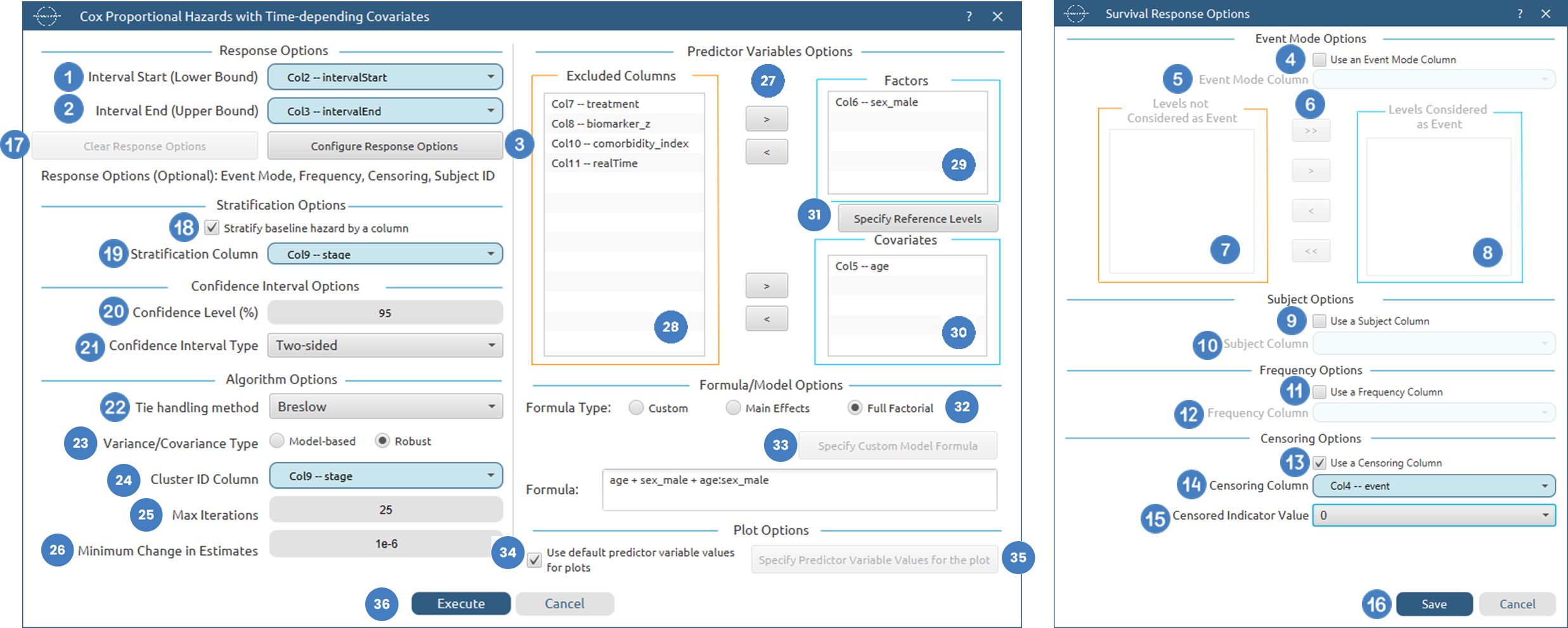
Output
The tables summarizing the survival analysis results for the cox proportional hazards model with time-dependent covariates are shown in the output spreadsheet. In addition, a pop-up window displays the survival curve for each of the selected sets of covariate settings.
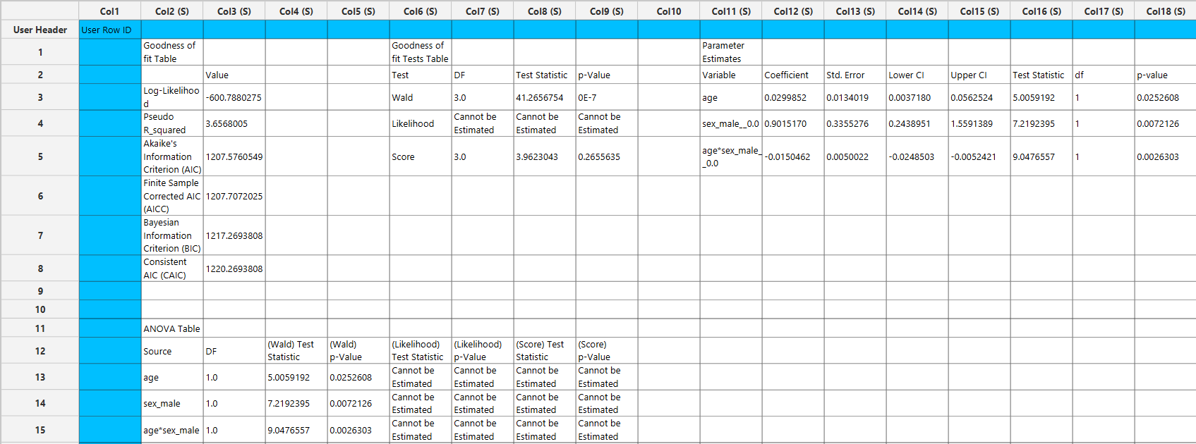
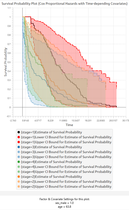
Configure Response Options
The Response Options dialog window allows the user to configure optional information related to how survival outcomes are interpreted and processed before fitting the Cox model. These options extend the basic time input by defining event types, censoring behavior, frequency weights, and model-specific time structure.
There are two variants of this dialog window: one for the fixed covariates model and one for the time-varying covariates model.
-
For the Cox model with fixed covariates, the dialog includes Event Mode Options, Entry Time Options, Frequency Options, and Censoring Options. The entry time option allows the user to specify delayed entry or left truncation, where subjects enter the risk set after time zero. The censoring options also allow the user to censor observations at or above a specified threshold value.
-
For the Cox model with time-varying covariates, the dialog includes Event Mode Options, Subject Options, Frequency Options, and Censoring Options. The subject option allows the user to specify a subject ID column, which is used to identify repeated intervals belonging to the same subject. When provided, the method checks that intervals for each subject do not overlap, that each subject has no more than one event, and that any event occurs only in the final interval for that subject.
The Event Mode Options section allows the user to specify an event mode column when the dataset contains different types of events. The levels of this column can be moved between the “Levels not Considered as Event” and “Levels Considered as Event” lists. Only observations with selected event levels are included as events according to the analysis configuration.
The Frequency Options section allows the user to specify a frequency column containing non-negative numerical values. This column represents the number of identical observations associated with each row. If no frequency column is selected, each row is treated as one observation.
The Censoring Options section allows the user to specify a censoring column and the value that identifies censored observations. The censoring column may be numerical or textual. In the fixed covariates variant, the user may also choose to censor times at or above a specified threshold value.
These options are optional. If they are not configured, the model assumes that all rows represent single observations, all included rows correspond to the selected event structure, and no additional censoring, frequency weighting, entry-time adjustment, or subject-level validation is applied.
Dialog window components (Fixed Covariates Model)
| Use an Event Mode Column | Enable this option to include an event mode column in the analysis. |
| Event Mode Column | If the Use an Event Mode Column option is enabled, specify the column containing event mode information. |
| Levels not Considered as Event/Levels Considered as Event | Manually select which levels should be treated as events from the available levels of the Event Mode Column. Use the arrow buttons to move levels between the two lists. Single-arrow buttons move selected levels, while double-arrow buttons move all levels. At least one level must be selected as an event. |
| Use an Entry Time Column | Enable this option to include an entry time column in the analysis. This is used only in the fixed covariates model to account for delayed entry (left truncation), where subjects enter the risk set after time zero. |
| Entry Time Column | If the Use an Entry Time Column option is enabled, select the column containing entry time values for each observation. This column must be numerical, contain non-negative values, and each entry time must be less than or equal to the corresponding event or censoring time. |
| Use a Frequency Column | Enable this option to include a frequency column in the analysis. |
| Frequency Column | If the Use a Frequency Column option is enabled, select the column containing frequency information for each observation. This column must be numerical and contain non-negative values. |
| Use a Censoring Column | Enable this option to include a censoring column in the analysis. |
| Censoring Column | If the Use a Censoring Column option is enabled, select the column containing censoring information for each observation. This column must be categorical and may be either numerical or textual. |
| Censoring Indicator Value | If a censoring column is used, specify which of its two levels represents a censored observation. |
| Censor times at or above a value | Enable this option to treat all time values greater than or equal to a specified threshold as censored. |
| Censoring Threshold Value | If the Censor times at or above a value option is enabled, specify the value above or equal to which observations will be treated as censored. |
Dialog window components (Time-Dependent Covariates Model)
| Use an Event Mode Column | Enable this option to include an event mode column in the analysis. |
| Event Mode Column | If the Use an Event Mode Column option is enabled, specify the column containing event mode information. |
| Levels not Considered as Event/Levels Considered as Event | Manually select which levels should be treated as events from the available levels of the Event Mode Column. Use the arrow buttons to move levels between the two lists. Single-arrow buttons move selected levels, while double-arrow buttons move all levels. At least one level must be selected as an event. |
| Use a Subject Column | Enable this option to include a subject identifier column in the analysis. This option is used only in the time-dependent covariates model to link multiple rows belonging to the same subject. |
| Subject Column | If the Use a Subject Column option is enabled, select the column identifying subjects. This column is used to validate that intervals for each subject do not overlap, that each subject has at most one event, and that any event occurs only in the subject’s final interval. |
| Use a Frequency Column | Enable this option to include a frequency column in the analysis. |
| Frequency Column | If the Use a Frequency Column option is enabled, select the column containing frequency information for each observation. This column must be numerical and contain non-negative values. |
| Use a Censoring Column | Enable this option to include a censoring column in the analysis. |
| Censoring Column | If the Use a Censoring Column option is enabled, select the column containing censoring information for each observation. This column must be categorical and may be either numerical or textual. |
| Censoring Indicator Value | If a censoring column is used, specify which of its two levels represents a censored observation. |
Parametric Methods
Parametric methods in survival analysis are statistical techniques that assume a specific probability distribution for the time-to-event data. Common choices include exponential, Weibull, log-normal, and log-logistic distributions. By imposing a functional form on the survival distribution, these methods enable fully specified models for the survival, hazard, and cumulative hazard functions.
Because the underlying distribution is explicitly defined, parametric methods can provide more efficient and precise estimates when the chosen distribution adequately represents the data. However, they are more sensitive to model misspecification; incorrect distributional assumptions may lead to biased results and misleading inference.
Parametric methods are primarily used to:
- Estimate survival and hazard functions under an assumed distribution
- Provide smooth, continuous representations of survival behavior
- Extrapolate survival beyond the observed time range
- Incorporate censored observations within a likelihood-based framework (MLE)
- Compare candidate distributions to identify the best-fitting model
These methods are typically applied when there is theoretical or empirical justification for a specific distribution, or when smooth estimation and extrapolation are required beyond the observed data range.
Univariate Parametric Analysis (Right-Censoring)
The Univariate Parametric Analysis method is a parametric survival analysis technique used to estimate survival characteristics from right-censored time-to-event data by assuming that the observed survival times follow a specified probability distribution. Unlike non-parametric methods, which estimate the survival function directly from the data, this method fits a smooth mathematical distribution to the observed survival times and uses the fitted distribution to estimate survival, hazard, and failure behavior.
This method is univariate, meaning that it models the distribution of the time variable itself without including predictor variables or covariate effects. It is useful when the goal is to describe the survival pattern of a sample, compare survival behavior across groups, or obtain smooth fitted survival and hazard curves under a chosen distributional assumption.
The user specifies a Time Column containing non-negative numerical values representing the observed event or censoring time for each subject. The user also selects an Expected Distribution, which defines the assumed parametric form of the survival model. Available distributions include Weibull, 3-Parameter Weibull, Exponential, 2-Parameter Exponential, Normal, Lognormal, 3-Parameter Lognormal, Logistic, Loglogistic, 3-Parameter LogLogistic, and Smallest Extreme Value. More on Available Distributions
For a fitted parametric distribution, the survival function is expressed as:
where \(F(t)\) is the cumulative distribution function of the selected distribution. The corresponding probability of failure by time \(t\) is:
The hazard function describes the instantaneous event rate at time t, conditional on survival up to that time:
where \(f(t)\) is the probability density function of the selected distribution and \(S(t)\) is the survival function.
Right-censored observations are incorporated by identifying observations for which the event has not occurred by the recorded time. These observations contribute information that the true event time exceeds the censoring time. If a censoring column is specified, the selected censoring indicator value determines which rows are treated as censored. The user may also choose to censor all observations with time values greater than or equal to a specified threshold value. Observations not marked as censored are treated as event observations.
The method supports two estimation approaches: Maximum Likelihood Estimation and Least Squares. Maximum Likelihood Estimation is the default method and estimates the distribution parameters by maximizing the likelihood of the observed event and censored data. Under right-censoring, uncensored observations contribute through the density function, while censored observations contribute through the survival function. The likelihood can be expressed as:
where θ represents the distribution parameters, \(t_i\) is the observed time, and \(\delta_i\) indicates whether the observation is an event.
The Least Squares option estimates the distribution parameters by fitting the selected distribution to transformed empirical survival information. This approach provides an alternative to likelihood-based estimation, although it may be less appropriate when censoring is substantial.
Optional frequency weights may be included to represent repeated identical observations. If no frequency column is selected, each row is treated as one observation. An event mode column may also be specified when different event types are present; only the selected event levels are considered in the analysis. In addition, a grouping column may be used to fit the selected parametric model separately for each group, while also producing results for the full sample.
The output includes a Parameter Estimates Table, which reports the fitted distribution parameters. When Maximum Likelihood Estimation is used, standard errors and confidence interval bounds are also reported according to the selected confidence level and confidence interval type. The output also includes estimated distribution characteristics derived from the fitted model.
The results are visualized using a fitted parametric survival probability plot. Unlike the Kaplan–Meier curve, which is stepwise, the parametric survival curve is smooth because it is generated from the selected fitted distribution. Optionally, the user may also generate the fitted hazard function plot and the cumulative probability of failure plot. When grouping is enabled, the method produces corresponding fitted curves for the full sample and for each group separately.
Use the Univariate Parametric Analysis (Right-Censoring) method when the survival data can reasonably be described by a known distribution, when smooth survival and hazard estimates are desired, or when extrapolation beyond the observed event times is needed.
Use the Univariate Parametric Analyis (Right-Censoring) method by browsing in the top ribbon:
Statistics \(\rightarrow\) Survival Analysis \(\rightarrow\) Parametric \(\rightarrow\) Univariate Parametric Analyis (Right-Censoring) |
Input
The Univariate Parametric Analyis (Right-Censoring) requires at least one column of numerical data to be specified in the input datasheet. The required input is a time variable column containing non-negative numerical values, representing the observed time-to-event or time-to-censoring for each subject. In addition to the time variable, several optional inputs may be provided to extend the functionality of the analysis. A censoring column may be specified as a variable, either numerical or textual, indicating whether each observation corresponds to an event or a censored case. A frequency column may also be included, consisting of non-negative numerical values that represent the number of identical observations associated with each row; if this column is not provided, each row is treated as a single observation by default. Furthermore, an event mode column may be defined, which can be either numerical or textual, and is used to distinguish between different types of events depending on the analysis configuration. Finally, a grouping column can be specidied as a categorical variable, either numerical or textual, indicating the group membership of each observation. All input columns must be of consistent type and should not contain invalid or missing values, as this may prevent the method from executing correctly.
Configuration
| Time Column | Select the column corresponding to the observed time-to-event or time-to-censoring for each subject. This column must be numerical and contain non-negative values. |
| Expected Distribution | Select the expected distribution of the time column. Available options include: Weibull, Smallest Extreme Value, 3-Parameter Weibull, Exponential, 2-Parameter Exponential, Normal, Lognormal, 3-Parameter Lognormal, Logistic, LogLogistic, 3-Parameter LogLogistic. |
| Configure Event Mode Options | Use this button to open the Configure Event Mode Options window |
| Event Mode Column | Within the Configure Event Mode Options window, specify the column containing event mode information. |
| Levels not Considered as Event/Levels Considered as Event | Manually select which levels should be treated as events from the available levels of the Event Mode Column. Use the arrow buttons to move levels between the two lists. Single-arrow buttons move selected levels, while double-arrow buttons move all levels. At least one level must be selected as an event. |
| Clear Event Mode Options | Use this button to clear all selections related to event mode configuration. |
| Use a Frequency Column | Enable this option to include a frequency column in the analysis. |
| Frequency Column | If the Use a Frequency Column option is enabled, select the column containing frequency information for each observation. This column must be numerical and contain non-negative values. |
| Use a Censoring Column | Enable this option to include a censoring column in the analysis. |
| Censoring Column | If the Use a Censoring Column option is enabled, select the column containing censoring information for each observation. This column must be categorical and may be either numerical or textual. |
| Censoring Indicator Value | If a censoring column is used, specify which of its two levels represents a censored observation. |
| Censor times at or above a value | Enable this option to treat all time values greater than or equal to a specified threshold as censored. |
| Censoring Threshold Value | If the Censor times at or above a value option is enabled, specify the value above or equal to which observations will be treated as censored. |
| Use a Grouping Column | Enable this option to include a grouping column in the analysis, allowing comparison of survival across different groups in the population. |
| Grouping Column | If the Use a Grouping Column option is enabled, select the column containing grouping information for each observation. This column must be categorical. |
| Estimation Method | Select the method used to estimate the distribution parameters. Available options include Maximum Likelihood and Least Squares. Maximum Likelihood is the default method and supports censored observations and confidence interval estimation. The Least Squares method estimates parameters by fitting the selected distribution to empirical survival information and does not allow computation of confidence intervals. |
| Max Iterations | Specify the maximum number of iterations allowed for the optimization algorithm when Maximum Likelihood estimation is selected. Higher values may be required for difficult convergence cases. Default value is 25. |
| Minimum Change in Estimates | Define the convergence threshold for the optimization algorithm when Maximum Likelihood estimation is selected. The algorithm stops when the change in parameter estimates between iterations falls below this value. Default value is 1e−6. |
| Confidence Level (%) | Specify the confidence level of the analysis. Values should range from 0 to 100 and correspond to percentages. Default value is set to 95. |
| Confidence Interval Type | Select the type of confidence interval to compute. Available options include: Two-sided, Lower Bound, Upper Bound. |
| Hazard Function Plot | Enable this option to generate a plot of the estimated hazard function over time. |
| Cumulative Probability of Failure Plot | Enable this option to generate a plot of the estimated cumulative probability of failure over time. |
Output
The output of the Univariate Parametric Analysis is presented in a structured spreadsheet containing summary tables of the fitted distribution parameters and derived survival characteristics. The spreadsheet includes a Parameter Estimates Table, which reports the estimated parameters of the selected distribution (e.g., shape, scale, location, or threshold depending on the distribution). When the Maximum Likelihood Estimation (MLE) method is used, the table also includes standard errors and confidence interval bounds at the selected confidence level. If the Least Squares method is selected, only the parameter estimates are reported, as confidence intervals and standard errors are not computed. In addition, the output includes a Characteristics Table, which provides derived quantities from the fitted distribution, such as measures related to survival behavior (e.g., quantiles or other distribution-specific characteristics), along with confidence intervals when available. If a grouping column is specified, the spreadsheet first presents the results for the full sample, followed by separate parameter and characteristics tables for each group.
A pop-up window displays the fitted survival probability curve, which is a smooth curve derived from the selected parametric distribution. Confidence interval bounds are shown when available (i.e., under MLE). Unlike the Non-Parametric and Semi-Parametric methods, this curve is continuous and defined over the entire time range.Optionally, the user may also generate the hazard function plot and the cumulative probability of failure plot, both derived from the fitted distribution. When grouping is enabled, the plots include the overall fitted curve as well as separate curves for each group, allowing comparison of survival behavior across groups under the assumed distribution.
Example
Input
In the input datasheet the requirement is to specify at least one numerical column and insert the appropriate data, as shown below.
Configuration
- Select
Statistics→Survival Analysis→Non-Parametric→Univariate Parametric Analysis (Right-Censoring). - Select the
Time Column[1]. This column should contain non-negative numeric values. - Select the
Expected Distribution[2] of the time column from the available options. - Optionally click on the
Configure Event Mode Options[3] button to select anEvent Mode Column[4] and use the arrow buttons [5] to select the levels that should be accounted for in the analysis by moving them between theLevels not Considered as Event[6] andLevels Considered as Event[7] lists.SaveorCancelany changes made using the appropriate buttons [8]. - Once you have configured some Event Mode Options you can optionally use the
Clear Event Mode Options[9] button to erase any selections made. - Select/tick to
Use a Frequency Column[10]. - If the
Use a Frequency Columnoption is selected, specify aFrequency Column[11]. This column should contain non-negative numeric values. - Select/tick to
Use a Censoring Column[12]. - If the
Use a Censoring Columnoption is selected, specify aCensoring Column[13] and the value of this column that should be theCensored Indicator Value[14]. - Select/tick to
Censor times at or above a value[15]. - If the ``Censor times at or above a value
option is selected, specify aCensoring Thresholdd Value`[16] above which events are considered censored. - Select/tick to
Use a Grouping Column[17]. - If the
Use a Grouping Columnoption is selected, specify aGrouping Column[18]. This column should be categorical, either textual or numerical. - Select the desired
Estimation Method[19]. - Specify the
Max Iterations[20] of the iterative algorithm to perform and theMinimum Change in Parameter Estimates[21]. - If the Maximum Likelihood
Estimation Methodis selected, specify theConfidence Level(%) [22] for Confidence Intervals and the desiredConfidence Interval Type[23]. - Optionally select/tick to calculate and present the
Hazard Function Plot[24] and theCumulative Probability of Failure Plot[25]. - Click on the
Executebutton [26] to perform the Univariate Parametric Analysis (Right-Censoring) method.
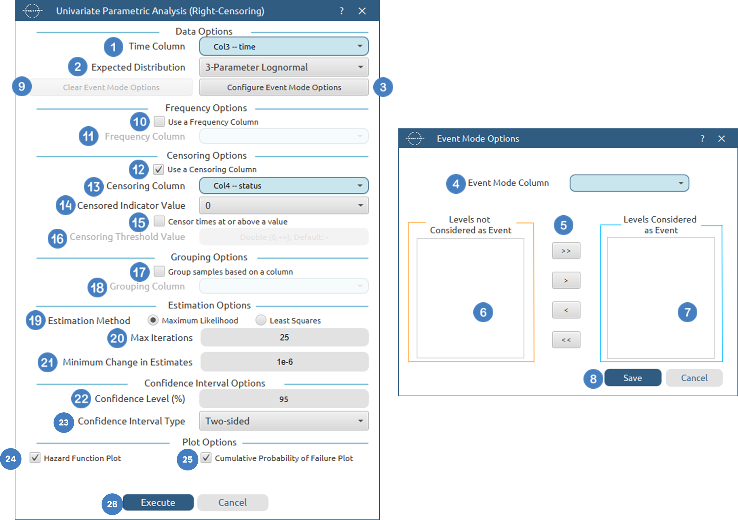
Output
The tables summarizing the survival analysis results for the non grouped dataset and each grouping level are shown in the output spreadsheet. In addition, a pop-up window displays the survival curve and, if selected, the hazard function and cumulative probability of failure plots.
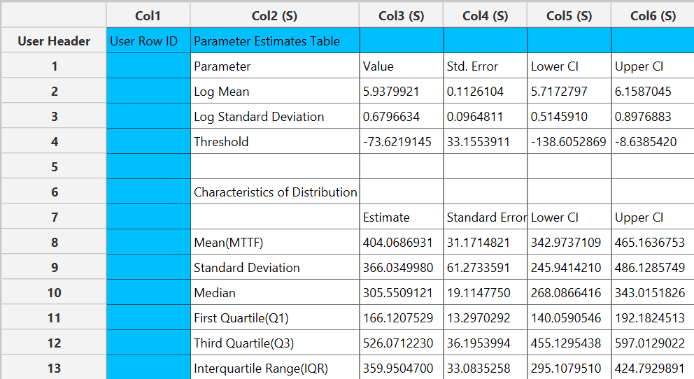
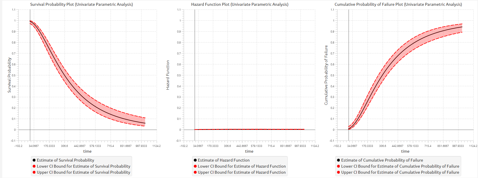
Univariate Parametric Analysis (Interval-Censoring)
The Univariate Parametric Analysis (Interval-Censoring) method is a parametric survival analysis technique used to estimate survival characteristics from interval-censored time-to-event data by assuming that the underlying survival times follow a specified probability distribution. Unlike right-censored survival analysis, where the exact censoring time is known, interval-censoring occurs when the event is only known to have occurred within a time interval bounded by a lower and upper observation time.
This method is univariate, meaning that it models the distribution of the survival time itself without incorporating predictor variables or covariates. It is useful when the goal is to describe the survival behavior of a sample, estimate smooth survival and hazard functions, or model failure behavior when exact event times are not directly observed.
The user specifies an Interval Start (Lower Bound) column and an Interval End (Upper Bound) column containing the lower and upper bounds of the interval in which the event occurred. Exact observations may also be represented by rows where the lower and upper bounds are equal. Left-censored observations may be represented by intervals of the form \((−∞,u]\), while right-censored observations may be represented by intervals of the form \([l,+∞)\).
The user also selects an Expected Distribution, which defines the assumed parametric form of the survival model. Available distributions include Weibull, 3-Parameter Weibull, Exponential, 2-Parameter Exponential, Normal, Lognormal, 3-Parameter Lognormal, Logistic, Loglogistic, 3-Parameter LogLogistic, and Smallest Extreme Value. More on Available Distributions
For a fitted parametric distribution, the survival function is expressed as:
where F(t) is the cumulative distribution function of the selected distribution. The corresponding cumulative probability of failure by time t is:
The hazard function describes the instantaneous event rate at time t conditional on survival up to time t:
where \(f(t)\) is the probability density function of the selected distribution.
The method supports two estimation approaches: Maximum Likelihood Estimation and Least Squares.
Maximum Likelihood Estimation is the default method and estimates the distribution parameters by maximizing the likelihood of the observed interval-censored data. For interval-censored observations, the contribution of each observation corresponds to the probability that the event time lies within the observed interval:
where \(l_i\) and \(u_i\) represent the lower and upper bounds of the interval for observation i and θ denotes the distribution parameters.
Special cases are handled naturally:
Exact observations contribute through:
Right-censored observations contribute through:
Left-censored observations contribute through:
The Least Squares option estimates the distribution parameters by fitting the selected distribution to transformed empirical survival information derived from the interval-censored data. This approach provides an alternative to likelihood-based estimation, although Maximum Likelihood Estimation is generally preferred for interval-censored survival analysis.
Optional frequency weights may be included to represent repeated identical observations. If no frequency column is selected, each row is treated as one observation.
An Event Mode column may also be specified when different event types are present. Only the selected event levels are included as events in the analysis, while other rows are excluded according to the selected event mode configuration.
In addition, a Grouping Column may be specified to fit the selected parametric model separately for each group while also producing results for the complete dataset.
The output includes a Parameter Estimates Table, which reports the fitted distribution parameters. When Maximum Likelihood Estimation is used, standard errors, confidence intervals, and inferential statistics are also reported according to the selected confidence level and confidence interval type.
The method also produces estimated distribution characteristics derived from the fitted model, including survival probabilities, cumulative failure probabilities, hazard functions, and other distribution-specific characteristics.
The fitted results are visualized using smooth parametric curves generated from the selected distribution. Optionally, the user may generate:
- A fitted Hazard Function Plot
- A fitted Cumulative Probability of Failure Plot
When grouping is enabled, separate fitted curves are produced for each group in addition to the full-sample results.
Use the Univariate Parametric Analysis (Interval-Censoring) method when the exact event times are not directly observed but are known to lie within intervals, when smooth parametric survival estimates are desired, or when extrapolation beyond the observed intervals is required.
Use the Univariate Parametric Analysis (Interval-Censoring) method by browsing in the top ribbon:
Statistics \(\rightarrow\) Survival Analysis \(\rightarrow\) Parametric \(\rightarrow\) Univariate Parametric Analyis (Interval-Censoring) |
Input
The Univariate Parametric Analysis (Interval-Censoring) requires at least two columns of numerical data to be specified in the input datasheet. The required inputs are an interval start (lower bound) column and an interval end (upper bound) column containing non-negative numerical values, representing the lower and upper bounds of the interval within which the event occurred for each subject. Exact observations may be represented by rows where the lower and upper bounds are equal. Left-censored and right-censored observations may also be represented through appropriate interval bounds depending on the analysis configuration. In addition to the interval bounds, several optional inputs may be provided to extend the functionality of the analysis. A frequency column may also be included, consisting of non-negative numerical values that represent the number of identical observations associated with each row; if this column is not provided, each row is treated as a single observation by default. Furthermore, an event mode column may be defined, which can be either numerical or textual, and is used to distinguish between different types of events depending on the analysis configuration. Finally, a grouping column can be specified as a categorical variable, either numerical or textual, indicating the group membership of each observation. All input columns must be of consistent type and should not contain invalid or missing values, as this may prevent the method from executing correctly. In addition, the lower bound must be less than or equal to the corresponding upper bound for every observation.
Configuration
| Interval Start (Lower Bound) | Select the column corresponding to the lower bound of the interval for each subject. This column must be numerical and contain non-negative values. |
| Interval End (Upper Bound) | Select the column corresponding to the upper bound of the interval for each subject. This column must be numerical and contain non-negative values. For each row the upper bound should be larger or equal to the lower bound. |
| Expected Distribution | Select the expected distribution of the time column. Available options include: Weibull, Smallest Extreme Value, 3-Parameter Weibull, Exponential, 2-Parameter Exponential, Normal, Lognormal, 3-Parameter Lognormal, Logistic, LogLogistic, 3-Parameter LogLogistic. |
| Configure Event Mode Options | Use this button to open the Configure Event Mode Options window |
| Event Mode Column | Within the Configure Event Mode Options window, specify the column containing event mode information. |
| Levels not Considered as Event/Levels Considered as Event | Manually select which levels should be treated as events from the available levels of the Event Mode Column. Use the arrow buttons to move levels between the two lists. Single-arrow buttons move selected levels, while double-arrow buttons move all levels. At least one level must be selected as an event. |
| Clear Event Mode Options | Use this button to clear all selections related to event mode configuration. |
| Use a Frequency Column | Enable this option to include a frequency column in the analysis. |
| Frequency Column | If the Use a Frequency Column option is enabled, select the column containing frequency information for each observation. This column must be numerical and contain non-negative values. |
| Use a Grouping Column | Enable this option to include a grouping column in the analysis, allowing comparison of survival across different groups in the population. |
| Grouping Column | If the Use a Grouping Column option is enabled, select the column containing grouping information for each observation. This column must be categorical. |
| Estimation Method | Select the method used to estimate the distribution parameters. Available options include Maximum Likelihood and Least Squares. Maximum Likelihood is the default method and supports censored observations and confidence interval estimation. The Least Squares method estimates parameters by fitting the selected distribution to empirical survival information and does not allow computation of confidence intervals. |
| Max Iterations | Specify the maximum number of iterations allowed for the optimization algorithm when Maximum Likelihood estimation is selected. Higher values may be required for difficult convergence cases. Default value is 25. |
| Minimum Change in Estimates | Define the convergence threshold for the optimization algorithm when Maximum Likelihood estimation is selected. The algorithm stops when the change in parameter estimates between iterations falls below this value. Default value is 1e−6. |
| Confidence Level (%) | Specify the confidence level of the analysis. Values should range from 0 to 100 and correspond to percentages. Default value is set to 95. |
| Confidence Interval Type | Select the type of confidence interval to compute. Available options include: Two-sided, Lower Bound, Upper Bound. |
| Hazard Function Plot | Enable this option to generate a plot of the estimated hazard function over time. |
| Cumulative Probability of Failure Plot | Enable this option to generate a plot of the estimated cumulative probability of failure over time. |
Output
The output of the Univariate Parametric Analysis is presented in a structured spreadsheet containing summary tables of the fitted distribution parameters and derived survival characteristics. The spreadsheet includes a Parameter Estimates Table, which reports the estimated parameters of the selected distribution (e.g., shape, scale, location, or threshold depending on the distribution). When the Maximum Likelihood Estimation (MLE) method is used, the table also includes standard errors and confidence interval bounds at the selected confidence level. If the Least Squares method is selected, only the parameter estimates are reported, as confidence intervals and standard errors are not computed. In addition, the output includes a Characteristics Table, which provides derived quantities from the fitted distribution, such as measures related to survival behavior (e.g., quantiles or other distribution-specific characteristics), along with confidence intervals when available. If a grouping column is specified, the spreadsheet first presents the results for the full sample, followed by separate parameter and characteristics tables for each group.
A pop-up window displays the fitted survival probability curve, which is a smooth curve derived from the selected parametric distribution. Confidence interval bounds are shown when available (i.e., under MLE). Unlike the Non-Parametric and Semi-Parametric methods, this curve is continuous and defined over the entire time range.Optionally, the user may also generate the hazard function plot and the cumulative probability of failure plot, both derived from the fitted distribution. When grouping is enabled, the plots include the overall fitted curve as well as separate curves for each group, allowing comparison of survival behavior across groups under the assumed distribution.
Example
Input
In the input datasheet the requirement is to specify at least two numerical column and insert the appropriate data, as shown below.
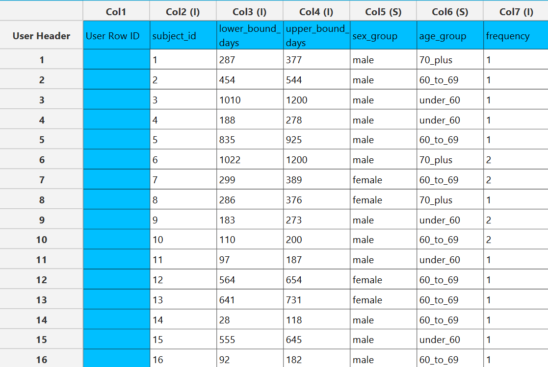
Configuration
- Select
Statistics→Survival Analysis→Non-Parametric→Univariate Parametric Analysis (Interval-Censoring). - Select the
Interval Start (Lower Bound)[1]. This column should contain non-negative numeric values. - Select the
Interval End (Upper Bound)[2]. This column should contain non-negative numeric values. - Select the
Expected Distribution[3] of the time column from the available options. - Optionally click on the
Configure Event Mode Options[4] button to select anEvent Mode Column[5] and use the arrow buttons [6] to select the levels that should be accounted for in the analysis by moving them between theLevels not Considered as Event[7] andLevels Considered as Event[8] lists.SaveorCancelany changes made using the appropriate buttons [9]. - Once you have configured some Event Mode Options you can optionally use the
Clear Event Mode Options[10] button to erase any selections made. - Select/tick to
Use a Frequency Column[11]. - If the
Use a Frequency Columnoption is selected, specify aFrequency Column[12]. This column should contain non-negative numeric values. - Select/tick to
Use a Grouping Column[13]. - If the
Use a Grouping Columnoption is selected, specify aGrouping Column[14]. This column should be categorical, either textual or numerical. - Select the desired
Estimation Method[15]. - Specify the
Max Iterations[16] of the iterative algorithm to perform and theMinimum Change in Parameter Estimates[17]. - If the Maximum Likelihood
Estimation Methodis selected, specify theConfidence Level(%) [18] for Confidence Intervals and the desiredConfidence Interval Type[19]. - Optionally select/tick to calculate and present the
Hazard Function Plot[20] and theCumulative Probability of Failure Plot[21]. - Click on the
Executebutton [22] to perform the Univariate Parametric Analysis (Right-Censoring) method.
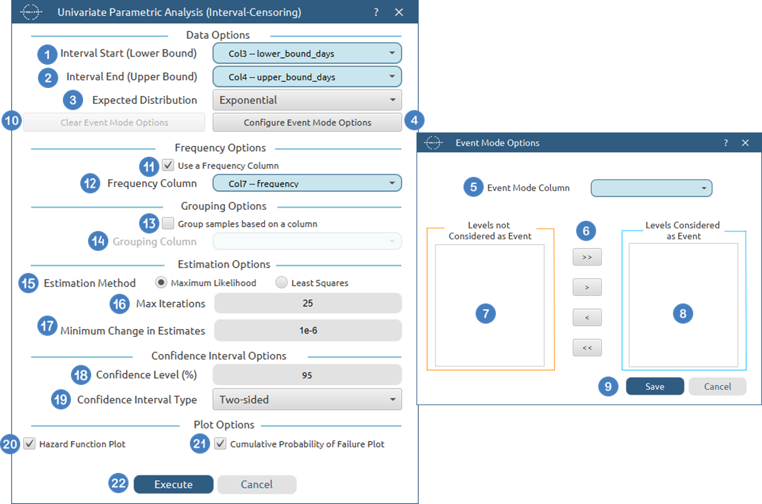
Output
The tables summarizing the survival analysis results for the non grouped dataset and each grouping level are shown in the output spreadsheet. In addition, a pop-up window displays the survival curve and, if selected, the hazard function and cumulative probability of failure plots.
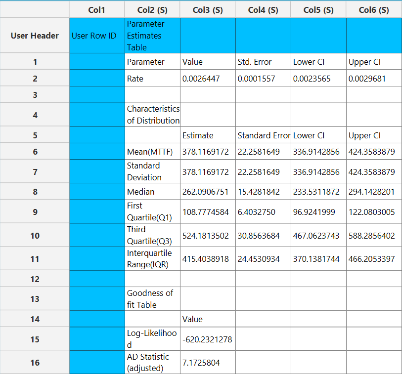
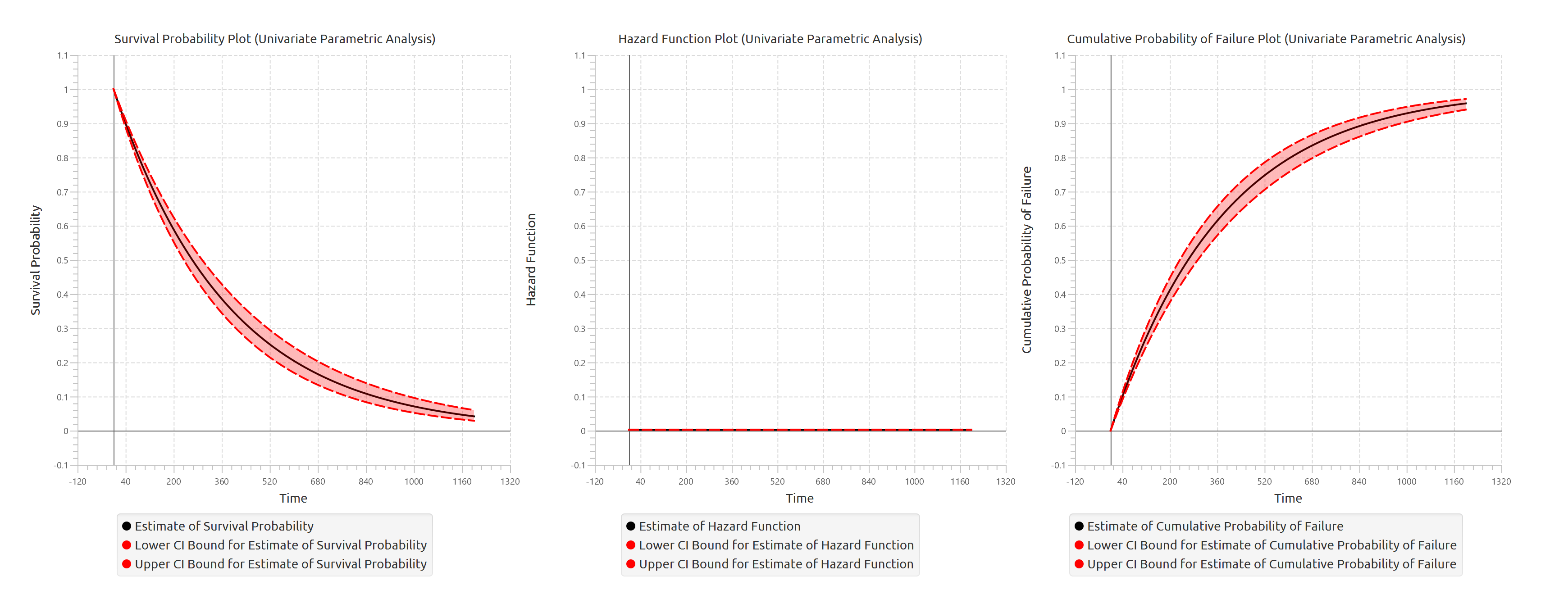
Accelerated Life Testing (Right-Censoring)
Accelerated Life Testing (ALT) with right-censored data is a parametric survival regression method used to model the effect of accelerating variables (stress variables) on the lifetime of a product, component, or system. Unlike semi-parametric survival models, ALT assumes that the survival times follow a specified probability distribution and directly models how stress conditions accelerate or decelerate the time-to-failure process.
The method relates survival time to predictor variables through an Accelerated Failure Time (AFT) formulation, where predictor variables act multiplicatively on the survival-time scale. In this framework, the survival time is modeled as a function of covariates, categorical factors, and a distribution-specific random error term.
The general Accelerated Failure Time formulation is:
where T is the survival time, x is the vector of predictor variables, β is the vector of estimated regression coefficients, σ is a scale parameter, and ϵ follows the error distribution associated with the selected parametric model.
For the Weibull, Exponential, Lognormal, and Loglogistic distributions, the model is formulated in terms of the logarithm of survival time log(T). In contrast, the Smallest Extreme Value, Normal, and Logistic distributions are modeled directly on the raw survival-time scale T.
Right-censored observations are incorporated by identifying observations for which the event has not occurred by the recorded time. These observations contribute information indicating that the true event time exceeds the observed censoring time. If a censoring column is specified, the selected censoring indicator value determines which rows are treated as censored. The user may additionally choose to administratively censor all observations with time values greater than or equal to a specified threshold value.
The method supports:
- Right-censored survival data
- Optional frequency weights
- Optional event-mode filtering
- Optional administrative censoring at a specified censoring value
- Continuous accelerating covariates and categorical factors
- Custom model formulas, main-effects models, and full factorial models
- Multiple accelerating-variable transformations
- Predicted survival curves for user-specified predictor patterns
The user specifies a Time Column containing non-negative numerical values representing the observed event or censoring time for each subject. The user also selects an Expected Distribution, which defines the assumed parametric form of the survival model. Available distributions include Weibull, Exponential, Normal, Lognormal, Logistic, Loglogistic and Smallest Extreme Value.
The model supports several accelerating-variable relationships that may be applied to numerical covariates before model fitting. Available accelerating relationships include:
- Linear
- Logarithmic
- Arrhenius
- Eyring
Only numerical covariates may be used as accelerating variables and transformed according to the selected accelerating relationship. Categorical factors are not transformed and are incorporated into the model through indicator-variable encoding.
The following accelerating-variable transformations are supported:
Linear Relationship
where x is the original covariate value.
Logarithmic Relationship
where \(x>0\).
Arrhenius Relationship
The Arrhenius relationship is commonly used for temperature-based accelerated testing. Input temperatures are assumed to be specified in degrees Celsius and are internally converted to Kelvin.
where x represents the temperature in degrees Celsius.
Eyring Relationship
The Eyring relationship is also commonly used for temperature-based accelerated testing. Input temperatures are assumed to be specified in degrees Celsius and are internally converted to Kelvin.
where x represents the temperature in degrees Celsius.
The method estimates model parameters using Maximum Likelihood Estimation. Under right-censoring, uncensored observations contribute through the probability density function, while censored observations contribute through the survival function. The likelihood function may be expressed as:
where θ represents the model parameters, \(t_i\) is the observed survival time for observation \(i\), and \(\delta_i\) indicates whether the observation corresponds to an event or a censored case.
The model output includes coefficient estimates, standard errors, confidence intervals, Wald statistics, degrees of freedom, and p-values for each fitted parameter. In addition, the model estimates the scale parameter of the selected distribution when applicable.
The method also provides model-level summaries, including the log-likelihood and goodness-of-fit statistics. Predicted survival curves may be generated for user-specified combinations of predictor values and factor levels.
This model is useful when the primary goal is to quantify how accelerating conditions affect product lifetime, estimate reliability under normal-use conditions, or extrapolate failure behavior beyond the observed testing environment.
Use the Accelerated Life Testing (Right-Censoring) method by browsing in the top ribbon:
Statistics \(\rightarrow\) Survival Analysis \(\rightarrow\) Parametric \(\rightarrow\) Accelerated Life Testing (Right-Censoring) |
Input
The Accelerated Life Testing (Right-Censoring) method requires at least two columns to be specified in the input datasheet: one numerical time column and at least one predictor variable. The time column must contain non-negative numerical values representing the observed time-to-event or time-to-censoring for each subject. Predictor variables may be specified either as categorical factors or numerical covariates and are used to model the effect of accelerating conditions on the survival distribution. In addition to the time variable and predictor variables, several optional inputs may be provided to extend the analysis. A censoring column may be specified as a numerical or textual variable indicating whether each observation corresponds to an event or a censored case. A frequency column may also be included, consisting of non-negative numerical values that represent the number of identical observations associated with each row; if this column is not provided, each row is treated as a single observation by default. Furthermore, an event mode column may be defined, using numerical or textual values to distinguish between different event types and determine which observations should be included in the analysis. The user may additionally specify an administrative censoring threshold value, where all observations with time values greater than or equal to the specified threshold are treated as censored. Categorical predictors may require reference levels, while numerical covariates may additionally be assigned accelerating-variable relationships including Linear, Logarithmic, Arrhenius, or Eyring transformations. Only numerical covariates may be used as accelerating variables. The selected predictors may be combined using a custom model formula, main-effects model, or full factorial model. All input columns must be of consistent type and should not contain invalid or missing values, as this may prevent the method from executing correctly.
Configuration
| Time Column | Select the column corresponding to the observed time-to-event or time-to-censoring for each subject. This column must be numerical and contain non-negative values. |
| Expected Distribution | Select the expected distribution of the time column. Available options include: Weibull, Smallest Extreme Value, 3-Parameter Weibull, Exponential, 2-Parameter Exponential, Normal, Lognormal, 3-Parameter Lognormal, Logistic, LogLogistic, 3-Parameter LogLogistic. |
| Configure Event Mode Options | Use this button to open the Configure Event Mode Options window |
| Event Mode Column | Within the Configure Event Mode Options window, specify the column containing event mode information. |
| Levels not Considered as Event/Levels Considered as Event | Manually select which levels should be treated as events from the available levels of the Event Mode Column. Use the arrow buttons to move levels between the two lists. Single-arrow buttons move selected levels, while double-arrow buttons move all levels. At least one level must be selected as an event. |
| Clear Event Mode Options | Use this button to clear all selections related to event mode configuration. |
| Use a Frequency Column | Enable this option to include a frequency column in the analysis. |
| Frequency Column | If the Use a Frequency Column option is enabled, select the column containing frequency information for each observation. This column must be numerical and contain non-negative values. |
| Use a Censoring Column | Enable this option to include a censoring column in the analysis. |
| Censoring Column | If the Use a Censoring Column option is enabled, select the column containing censoring information for each observation. This column must be categorical and may be either numerical or textual. |
| Censoring Indicator Value | If a censoring column is used, specify which of its two levels represents a censored observation. |
| Censor times at or above a value | Enable this option to treat all time values greater than or equal to a specified threshold as censored. |
| Censoring Threshold Value | If the Censor times at or above a value option is enabled, specify the value above or equal to which observations will be treated as censored. |
| Confidence Level (%) | Specify the confidence level of the analysis. Values should range from 0 to 100 and correspond to percentages. Default value is set to 95. |
| Confidence Interval Type | Select the type of confidence interval to compute. Available options include: Two-sided, Lower Bound, Upper Bound. |
| Max Iterations | Specify the maximum number of iterations allowed for the optimization algorithm (Newton-Raphson). Higher values may be required for complex models but will increase computation time. Default value is set to 25. |
| Minimum Change in Estimates | Define the convergence threshold for the optimization algorithm. The algorithm stops when the change in parameter estimates between iterations falls below this value. Default value is set to 1e-6. |
| Factors/ Covariates / Excluded columns | Select manually the columns that correspond to factors and the columns that correspond to covariates through the dialog window: Use the buttons to move columns between the Factors and Covariates list and Excluded Columns list. Single-arrow buttons will move all selected columns and double-arrow buttons will move all columns. At least one covariate column should be specified. |
| Specify Reference Levels | Specify the reference level for each of the categorical factors specified. The default option for each factor is its last level. |
| Formula Type | These options refer to the terms that will be included in the model. The Custom option allows the user to input a formula defining the exact terms to be included. The Main Effects option allows the analysis of a model that only includes all main effects and finally, the Full Factorial option includes both all main effects and all possible interaction terms to build a full model. |
| Specify Custom Model Formula | Specify the model formula used for the analysis if the Custom option is selected. The formula is created in the Custom Formula Creation dialog window by selecting factors and covariates and adding interaction terms up to the required order. Main effects of the included columns are always part of the model and cannot be excluded. |
| Use default prefictor variable values for plots | When enabled, predicted survival curves are generated using default values for predictors. These defaults are the reference levels for categorical factors and the midpoints of the observed ranges for numerical covariates. |
| Specify Predictor Variable Values for the plot | Define custom values for predictors to generate predicted survival curves. The user may specify up to 10 different sets of predictor values, and a separate survival curve will be produced for each set. |
Output
The output of the Accelerated Life Testing (Right-Censoring) method is presented in a structured spreadsheet containing multiple tables that summarize the fitted model, statistical inference, and overall model performance.
The main output includes a Parameter Estimates table, which reports the estimated regression coefficients for each predictor variable, along with their corresponding standard errors, confidence interval bounds at the selected confidence level, test statistics, degrees of freedom, and p-values. The table also includes the estimated scale parameter of the selected parametric distribution when applicable.
A Goodness-of-Fit table is also provided, summarizing key model diagnostics including the model log-likelihood. This measure may be used to assess overall model fit and compare competing accelerated life testing models fitted on the same dataset.
An ANOVA table is additionally generated, providing term-wise inference for each predictor variable and interaction term included in the fitted model. This table includes Wald, likelihood ratio, and score test statistics together with their corresponding degrees of freedom and p-values for each model term.
In addition to the tabular output, a pop-up window displays the predicted survival probability curves based on the fitted accelerated life testing model. These curves are computed using the estimated model coefficients and the selected parametric survival distribution. Confidence interval bounds are displayed according to the selected confidence interval type. When multiple sets of predictor values are specified, a separate survival curve (with confidence bounds) is plotted for each predictor configuration, allowing direct comparison of survival behavior under different accelerating conditions.
Example
Input
In the input datasheet the requirement is to specify at least two columns, from which at least one should be numerical and insert the appropriate data, as shown below.
Configuration
- Select
Statistics→Survival Analysis→Parametric→Accelerated Life Testing (Right-Censoring). - Select the
Time Column[1]. This column should contain non-negative numeric values. - Select the
Expected Distribution[2] of the time column from the available options. - Optionally click on the
Configure Event Mode Options[3] button to select anEvent Mode Column[4] and use the arrow buttons [6] to select the levels that should be accounted for in the analysis by moving them between theLevels not Considered as Event[5] andLevels Considered as Event[7] lists.SaveorCancelany changes made using the appropriate buttons [8]. - Once you have configured some Event Mode Options you can optionally use the
Clear Event Mode Options[9] button to erase any selections made. - Select/tick to
Use a Frequency Column[10]. - If the
Use a Frequency Columnoption is selected, specify aFrequency Column[11]. This column should contain non-negative numeric values. - Select/tick to
Use a Censoring Column[12]. - If the
Use a Censoring Columnoption is selected, specify aCensoring Column[13] and the value of this column that should be theCensored Indicator Value[14]. - Select/tick to
Censor times at or above a value[15]. - If the ``Censor times at or above a value
option is selected, specify aCensoring Thresholdd Value`[16] above which events are considered censored. - Specify the
Confidence Level(%) [17] for Confidence Intervals and the desiredConfidence Interval Type[18]. - Specify the
Max Iterations[19] of the iterative algorithm to perform and theMinimum Change in Parameter Estimates[20]. - Select the columns by clicking on the arrow buttons [21] and moving columns between the
Excluded Columns[22] andFactors[23] andCovariates[24] lists. - Optionally, specify
Specify Reference Levels[25] for the categorical factors. - Select the prefered
Formula Type[26]. Specify Custom Model Formula[27] for the analysis ifCustomoption is selected. How to specify a custom model formula?- Select/tick to
Use default predictor variable values for plots[28], otherwiseSpecify Predictor Variable Values for the plots[29]. - Click on the
Executebutton [30] to perform the Cox Proportional Hazards Model with Fixed Covariates.
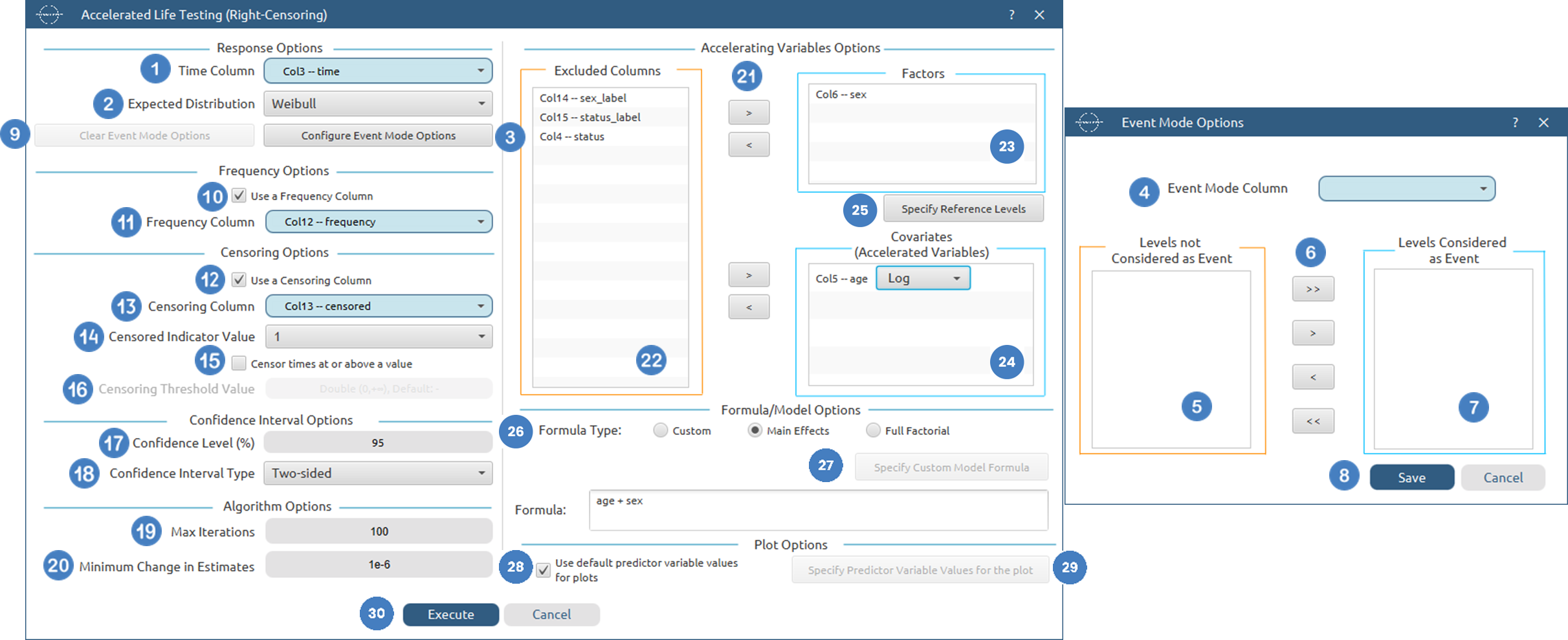
Output
The tables summarizing the Accelerated Life Testing (Right-Censoring) analysis results are shown in the output spreadsheet. These tables include the Goodness-of-Fit table, the Parameter Estimates table, and the ANOVA table containing Wald, likelihood ratio, and score tests for each model term.
In addition, a pop-up window displays the predicted survival probability curves generated from the fitted accelerated life testing model. Separate survival curves are produced for each selected set of predictor-variable settings, allowing direct comparison of survival behavior under different accelerating conditions. Confidence interval bounds are additionally displayed according to the selected confidence interval type.
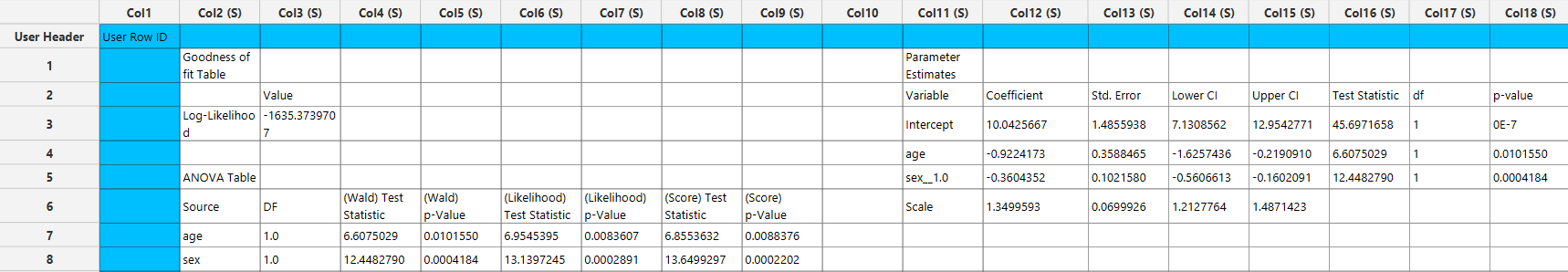
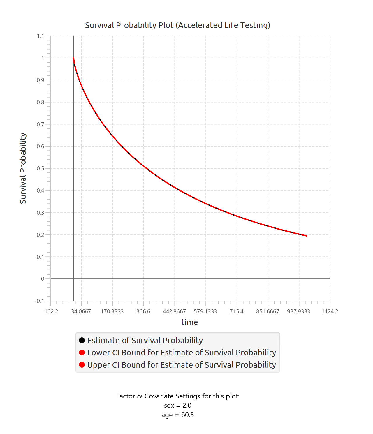
Accelerated Life Testing (Interval-Censoring)
Accelerated Life Testing (ALT) with interval-censored data is a parametric survival regression method used to model the effect of accelerating variables (stress variables) on the lifetime of a product, component, or system when the exact event times are not directly observed. Instead, the event is only known to have occurred within an interval bounded by a lower and upper observation time.
Unlike semi-parametric survival models, ALT assumes that the survival times follow a specified probability distribution and directly models how stress conditions accelerate or decelerate the time-to-failure process.
The method relates survival time to predictor variables through an Accelerated Failure Time (AFT) formulation, where predictor variables act multiplicatively on the survival-time scale. In this framework, the survival time is modeled as a function of covariates, categorical factors, and a distribution-specific random error term.
The general Accelerated Failure Time formulation is:
where T is the survival time, x is the vector of predictor variables, β is the vector of estimated regression coefficients, σ is a scale parameter, and ϵ follows the error distribution associated with the selected parametric model.
For the Weibull, Exponential, Lognormal, and Loglogistic distributions, the model is formulated in terms of the logarithm of survival time log(T). In contrast, the Smallest Extreme Value, Normal, and Logistic distributions are modeled directly on the raw survival-time scale T.
Interval-censored observations are incorporated by specifying lower and upper bounds for the interval within which the event occurred. Exact observations may be represented by intervals where the lower and upper bounds are equal. Left-censored observations may additionally be represented through intervals of the form (−∞,u], while right-censored observations may be represented through intervals of the form [l,+∞).
The method supports:
- Interval-censored survival data
- Optional frequency weights
- Optional event-mode filtering
- Continuous accelerating covariates and categorical factors
- Custom model formulas, main-effects models, and full factorial models
- Multiple accelerating-variable transformations
- Predicted survival curves for user-specified predictor patterns
The user specifies an Interval Start (Lower Bound) column and an Interval End (Upper Bound) column containing non-negative numerical values representing the interval within which the event occurred for each subject. The user also selects an Expected Distribution, which defines the assumed parametric form of the survival model. Available distributions include Weibull, Exponential, Normal, Lognormal, Logistic, Loglogistic and Smallest Extreme Value.
The model supports several accelerating-variable relationships that may be applied to numerical covariates before model fitting. Available accelerating relationships include:
- Linear
- Logarithmic
- Arrhenius
- Eyring
Only numerical covariates may be used as accelerating variables and transformed according to the selected accelerating relationship. Categorical factors are not transformed and are incorporated into the model through indicator-variable encoding.
The following accelerating-variable transformations are supported:
Linear Relationship
where x is the original covariate value.
Logarithmic Relationship
where \(x>0\).
Arrhenius Relationship
The Arrhenius relationship is commonly used for temperature-based accelerated testing. Input temperatures are assumed to be specified in degrees Celsius and are internally converted to Kelvin.
where x represents the temperature in degrees Celsius.
Eyring Relationship
The Eyring relationship is also commonly used for temperature-based accelerated testing. Input temperatures are assumed to be specified in degrees Celsius and are internally converted to Kelvin.
where x represents the temperature in degrees Celsius.
The method estimates model parameters using Maximum Likelihood Estimation. Under interval-censoring, each observation contributes the probability that the event time lies within the observed interval. The likelihood function may be expressed as:
where \(l_i\) and \(u_i\) denote the lower and upper interval bounds for observation i and θ represents the model parameters.
Special cases are handled naturally:
Exact observations contribute through:
Right-censored observations contribute through:
Left-censored observations contribute through:
The model output includes coefficient estimates, standard errors, confidence intervals, Wald statistics, degrees of freedom, and p-values for each fitted parameter. In addition, the model estimates the scale parameter of the selected distribution when applicable.
The method also provides model-level summaries, including the log-likelihood and goodness-of-fit statistics. Predicted survival curves may be generated for user-specified combinations of predictor values and factor levels.
This model is useful when the primary goal is to quantify how accelerating conditions affect product lifetime, estimate reliability under normal-use conditions, or extrapolate failure behavior beyond the observed testing environment when exact failure times are not directly observed.
Use the Accelerated Life Testing (Interval-Censoring) method by browsing in the top ribbon:
Statistics \(\rightarrow\) Survival Analysis \(\rightarrow\) Parametric \(\rightarrow\) Accelerated Life Testing (Interval-Censoring) |
Input
The Accelerated Life Testing (Interval-Censoring) method requires at least three columns to be specified in the input datasheet: one numerical lower-bound column, one numerical upper-bound column, and at least one predictor variable. The lower-bound and upper-bound columns must contain non-negative numerical values representing the interval within which the event occurred for each subject. Exact observations may be represented by rows where the lower and upper bounds are equal. Predictor variables may be specified either as categorical factors or numerical covariates and are used to model the effect of accelerating conditions on the survival distribution. In addition to the interval bounds and predictor variables, several optional inputs may be provided to extend the analysis. A frequency column may also be included, consisting of non-negative numerical values that represent the number of identical observations associated with each row; if this column is not provided, each row is treated as a single observation by default. Furthermore, an event mode column may be defined, using numerical or textual values to distinguish between different event types and determine which observations should be included in the analysis. Categorical predictors may require reference levels, while numerical covariates may additionally be assigned accelerating-variable relationships including Linear, Logarithmic, Arrhenius, or Eyring transformations. Only numerical covariates may be used as accelerating variables. The selected predictors may be combined using a custom model formula, main-effects model, or full factorial model. All input columns must be of consistent type and should not contain invalid or missing values, as this may prevent the method from executing correctly. In addition, the lower interval bound must be less than or equal to the corresponding upper interval bound for every observation.
Configuration
| Interval Start (Lower Bound) | Select the column corresponding to the lower bound of the interval for each subject. This column must be numerical and contain non-negative values. |
| Interval End (Upper Bound) | Select the column corresponding to the upper bound of the interval for each subject. This column must be numerical and contain non-negative values. For each row the upper bound should be larger or equal to the lower bound. |
| Expected Distribution | Select the expected distribution of the time column. Available options include: Weibull, Smallest Extreme Value, 3-Parameter Weibull, Exponential, 2-Parameter Exponential, Normal, Lognormal, 3-Parameter Lognormal, Logistic, LogLogistic, 3-Parameter LogLogistic. |
| Configure Event Mode Options | Use this button to open the Configure Event Mode Options window |
| Event Mode Column | Within the Configure Event Mode Options window, specify the column containing event mode information. |
| Levels not Considered as Event/Levels Considered as Event | Manually select which levels should be treated as events from the available levels of the Event Mode Column. Use the arrow buttons to move levels between the two lists. Single-arrow buttons move selected levels, while double-arrow buttons move all levels. At least one level must be selected as an event. |
| Clear Event Mode Options | Use this button to clear all selections related to event mode configuration. |
| Use a Frequency Column | Enable this option to include a frequency column in the analysis. |
| Frequency Column | If the Use a Frequency Column option is enabled, select the column containing frequency information for each observation. This column must be numerical and contain non-negative values. |
| Confidence Level (%) | Specify the confidence level of the analysis. Values should range from 0 to 100 and correspond to percentages. Default value is set to 95. |
| Confidence Interval Type | Select the type of confidence interval to compute. Available options include: Two-sided, Lower Bound, Upper Bound. |
| Max Iterations | Specify the maximum number of iterations allowed for the optimization algorithm (Newton-Raphson). Higher values may be required for complex models but will increase computation time. Default value is set to 25. |
| Minimum Change in Estimates | Define the convergence threshold for the optimization algorithm. The algorithm stops when the change in parameter estimates between iterations falls below this value. Default value is set to 1e-6. |
| Factors/ Covariates / Excluded columns | Select manually the columns that correspond to factors and the columns that correspond to covariates through the dialog window: Use the buttons to move columns between the Factors and Covariates list and Excluded Columns list. Single-arrow buttons will move all selected columns and double-arrow buttons will move all columns. At least one covariate column should be specified. |
| Specify Reference Levels | Specify the reference level for each of the categorical factors specified. The default option for each factor is its last level. |
| Formula Type | These options refer to the terms that will be included in the model. The Custom option allows the user to input a formula defining the exact terms to be included. The Main Effects option allows the analysis of a model that only includes all main effects and finally, the Full Factorial option includes both all main effects and all possible interaction terms to build a full model. |
| Specify Custom Model Formula | Specify the model formula used for the analysis if the Custom option is selected. The formula is created in the Custom Formula Creation dialog window by selecting factors and covariates and adding interaction terms up to the required order. Main effects of the included columns are always part of the model and cannot be excluded. |
| Use default prefictor variable values for plots | When enabled, predicted survival curves are generated using default values for predictors. These defaults are the reference levels for categorical factors and the midpoints of the observed ranges for numerical covariates. |
| Specify Predictor Variable Values for the plot | Define custom values for predictors to generate predicted survival curves. The user may specify up to 10 different sets of predictor values, and a separate survival curve will be produced for each set. |
Output
The output of the Accelerated Life Testing (Interval-Censoring) method is presented in a structured spreadsheet containing multiple tables that summarize the fitted model, statistical inference, and overall model performance.
The main output includes a Parameter Estimates table, which reports the estimated regression coefficients for each predictor variable, along with their corresponding standard errors, confidence interval bounds at the selected confidence level, test statistics, degrees of freedom, and p-values. The table also includes the estimated scale parameter of the selected parametric distribution when applicable.
A Goodness-of-Fit table is also provided, summarizing key model diagnostics including the model log-likelihood. This measure may be used to assess overall model fit and compare competing accelerated life testing models fitted on the same dataset.
An ANOVA table is additionally generated, providing term-wise inference for each predictor variable and interaction term included in the fitted model. This table includes Wald, likelihood ratio, and score test statistics together with their corresponding degrees of freedom and p-values for each model term.
In addition to the tabular output, a pop-up window displays the predicted survival probability curves based on the fitted accelerated life testing model. These curves are computed using the estimated model coefficients and the selected parametric survival distribution. Confidence interval bounds are displayed according to the selected confidence interval type. When multiple sets of predictor values are specified, a separate survival curve (with confidence bounds) is plotted for each predictor configuration, allowing direct comparison of survival behavior under different accelerating conditions.
Example
Input
In the input datasheet the requirement is to specify at least two columns, from which at least one should be numerical and insert the appropriate data, as shown below.
Configuration
- Select
Statistics→Survival Analysis→Parametric→Accelerated Life Testing (Right-Censoring). - Select the
Interval Start (Lower Bound)[1]. This column should contain non-negative numeric values. - Select the
Interval End (Upper Bound)[2]. This column should contain non-negative numeric values. - Select the
Expected Distribution[3] of the time column from the available options. - Optionally click on the
Configure Event Mode Options[4] button to select anEvent Mode Column[5] and use the arrow buttons [7] to select the levels that should be accounted for in the analysis by moving them between theLevels not Considered as Event[6] andLevels Considered as Event[8] lists.SaveorCancelany changes made using the appropriate buttons [9]. - Once you have configured some Event Mode Options you can optionally use the
Clear Event Mode Options[10] button to erase any selections made. - Select/tick to
Use a Frequency Column[11]. - If the
Use a Frequency Columnoption is selected, specify aFrequency Column[12]. This column should contain non-negative numeric values. - Specify the
Confidence Level(%) [13] for Confidence Intervals and the desiredConfidence Interval Type[14]. - Specify the
Max Iterations[15] of the iterative algorithm to perform and theMinimum Change in Parameter Estimates[16]. - Select the columns by clicking on the arrow buttons [17] and moving columns between the
Excluded Columns[18] andFactors[19] andCovariates[20] lists. - Optionally, specify
Specify Reference Levels[21] for the categorical factors. - Select the prefered
Formula Type[22]. Specify Custom Model Formula[23] for the analysis ifCustomoption is selected. How to specify a custom model formula?- Select/tick to
Use default predictor variable values for plots[24], otherwiseSpecify Predictor Variable Values for the plots[25]. - Click on the
Executebutton [26] to perform the Cox Proportional Hazards Model with Fixed Covariates.

Output
The tables summarizing the Accelerated Life Testing (Interval-Censoring) analysis results are shown in the output spreadsheet. These tables include the Goodness-of-Fit table, the Parameter Estimates table, and the ANOVA table containing Wald, likelihood ratio, and score tests for each model term.
In addition, a pop-up window displays the predicted survival probability curves generated from the fitted accelerated life testing model. Separate survival curves are produced for each selected set of predictor-variable settings, allowing direct comparison of survival behavior under different accelerating conditions. Confidence interval bounds are additionally displayed according to the selected confidence interval type.
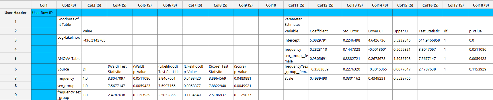
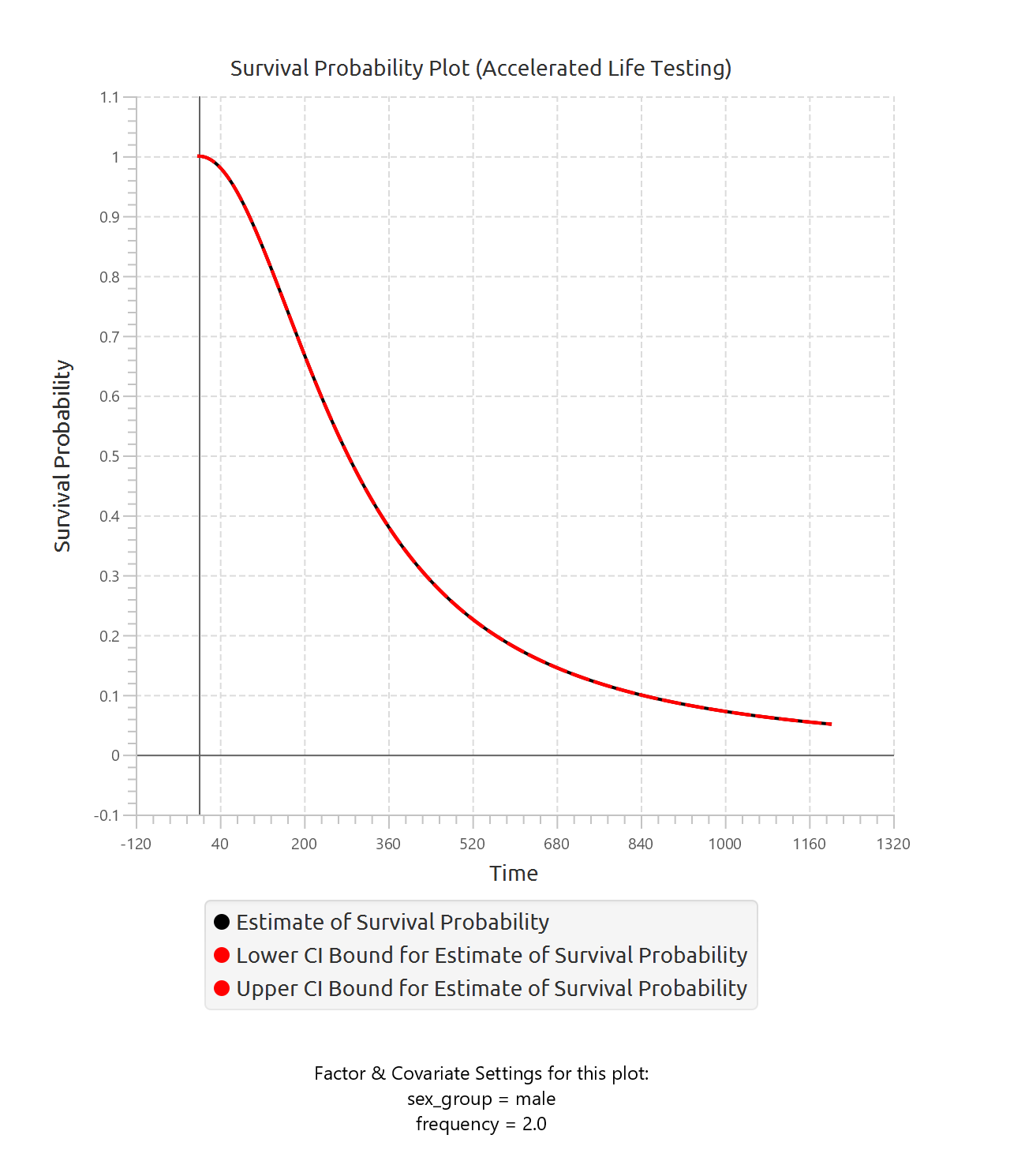
Distribution Equations and Estimated Parameters
The Parametric Methods fit one of the selected probability distributions to the observed time-to-event data. Each distribution is defined by its probability density function \(f(t)\), and the method estimates the unknown distribution parameters from the data.
Weibull Distribution
Estimated parameters:
- \(\beta\): Shape
- \(\eta\): Scale
3-Parameter Weibull Distribution
Estimated parameters:
- \(\beta\): Shape
- \(\eta\): Scale
- \(\gamma\): Threshold
Exponential Distribution
Estimated parameter:
- \(\lambda\): Rate
2-Parameter Exponential Distribution
Estimated parameters:
- \(\lambda\): Rate
- \(\gamma\): Threshold
Normal Distribution
Estimated parameters:
- \(\mu\): Location
- \(\sigma\): Scale
Lognormal Distribution
Estimated parameters:
- \(\mu\): Location
- \(\sigma\): Scale
3-Parameter Lognormal Distribution
Estimated parameters:
- \(\mu\): Location
- \(\sigma\): Scale
- \(\gamma\): Threshold
Logistic Distribution
Estimated parameters:
- \(\mu\): Location
- \(\sigma\): Scale
Loglogistic Distribution
Estimated parameters:
- \(\mu\): Location
- \(\sigma\): Scale
3-Parameter Loglogistic Distribution
Estimated parameters:
- \(\mu\): Location
- \(\sigma\): Scale
- \(\gamma\): Threshold
Smallest Extreme Value Distribution
Estimated parameters:
- \(\mu\): Location
- \(\sigma\): Scale
Anderson–Darling Test Statistic
The Anderson–Darling statistic is a goodness-of-fit measure used to evaluate how well the selected parametric distribution describes the observed data. Unlike goodness-of-fit measures that weight all portions of the distribution equally, the Anderson–Darling statistic places greater emphasis on the tails of the distribution, making it particularly sensitive to deviations in extreme values.
The statistic is calculated using the empirical plotting positions together with the cumulative probabilities predicted by the fitted distribution. Let \(z_i\) denote the ordered plotting positions and let \(F_i\) denote the corresponding fitted cumulative probabilities. The Anderson–Darling statistic is computed through an integrated discrepancy measure between the empirical and fitted distributions:
where the individual components are defined as:
where n is the sample size.
To ensure numerical stability, the plotting positions are internally constrained to lie within the interval:
with a small positive constant ϵ.
Smaller Anderson–Darling values indicate better agreement between the fitted distribution and the observed data, while larger values suggest poorer fit.
Pearson Correlation Coefficient for Probability Plots
It quantifies the strength of the linear relationship between the empirical quantiles of the observed data and the theoretical quantiles implied by the fitted distribution.
Before computing the correlation coefficient, the data and theoretical quantiles are transformed according to the selected parametric distribution. The transformation depends on the distributional form:
Logarithmic Transformation
For the Weibull, Exponential, Lognormal, and Loglogistic distributions:
where \(x>0\).
Shifted Logarithmic Transformation
For the 3-Parameter Weibull, 2-Parameter Exponential, 3-Parameter Lognormal, and 3-Parameter Loglogistic distributions:
where γ is the estimated threshold parameter and x>γ.
No Transformation
For the Normal, Logistic, and Smallest Extreme Value distributions:
After transformation, the Pearson correlation coefficient is computed between the transformed empirical quantiles and the transformed theoretical quantiles:
where \(x_i\) denotes the transformed empirical quantiles and \(y_i\) denotes the transformed theoretical quantiles.
Values of the Pearson correlation coefficient close to 1 indicate strong linear agreement between the empirical and theoretical quantiles and therefore suggest that the selected distribution provides a good fit to the observed data.
References
- Emmert-Streib, Frank, and Matthias Dehmer. “Introduction to survival analysis in practice.” Machine Learning and Knowledge Extraction 1, no. 3 (2019): 1013-1038. doi.org/10.3390/make1030058.
- Jenkins, Stephen P. “Survival analysis.” Unpublished manuscript, Institute for Social and Economic Research, University of Essex, Colchester, UK 42, no. 54-56 (2005): 1.
- Guo, Shenyang. Survival analysis. Oxford University Press, 2010.
- Hosmer Jr, D.W., Lemeshow, S. and May, S., 2008. Applied survival analysis: regression modeling of time-to-event data. John Wiley & Sons.
- Turnbull, Bruce W. “The empirical distribution function with arbitrarily grouped, censored and truncated data.” Journal of the Royal Statistical Society: Series B (Methodological) 38, no. 3 (1976): 290-295. doi.org/10.1111/j.2517-6161.1976.tb01597.x
- Turnbull, Bruce W. “Nonparametric estimation of a survivorship function with doubly censored data.” Journal of the American statistical association 69, no. 345 (1974): 169-173. doi.org/10.1080/01621459.1974.10480146
- Lin, Danyu Y., and Lee-Jen Wei. “The robust inference for the Cox proportional hazards model.” Journal of the American statistical Association 84, no. 408 (1989): 1074-1078.
- Andersen, Per Kragh, and Richard D. Gill. “Cox’s regression model for counting processes: a large sample study.” The annals of statistics (1982): 1100-1120.
- Genschel, U. and Meeker, W.Q. (2010). A Comparison of Maximum Likelihood and Median-Rank Regression for Weibull Estimation. Quality Engineering, 22(4): 236–255.
Version History
Introduced in Isalos Analytics Platform v2.0.3
Instructions last updated on May 2026