Bio

Biotransformation functions apply mathematical transformations to expression data matrices, preparing them for downstream analyses such as differential expression, dimensionality reduction, clustering, and visualisation. They are primarily used in bioinformatics and genomics workflows to stabilise variance, compress dynamic range, and bring measurements onto a biologically meaningful scale. ¹

Log2 Transformation
Log10 Transformation
VST
RLog
DESeq
Post Process DESeq
Normalize Between Arrays
Limma
Voom
See also
References
Version History

Log2 Transformation

The Log2 Transformation applies the element-wise function

\[f(x) = \log_2(x + c)\]

where c is a user-defined pseudo-count (default 1). The pseudo-count is added before the logarithm to prevent log₂(0) = −∞ for zero-count values and to handle near-zero measurements gracefully. This transformation is the standard preprocessing step in microarray analysis (limma log₂-intensity pipelines) and is widely used before RNA-Seq visualisation, PCA, and clustering to compress the large dynamic range of raw count data. ²>

The transformation is applied only to the columns explicitly moved to the Included Columns list; all other columns are passed through to the output unchanged.

Pre-validation

Before any value is transformed the algorithm checks that x + c > 0 for every cell in every selected column. If any column contains a value where x + c ≤ 0 the execution is aborted and an error message lists the offending columns. The pseudo-count should be increased, or the data pre-filtered, to resolve this.

Use the Log2 Transformation biotransformation function by browsing in the top ribbon:

Data Transformation $\rightarrow$ Biotransformation $\rightarrow$ Log2 Transformation

Input

The data input should consist of numerical instances without missing values in the columns to be transformed. At least 1 complete numerical column is required. Non-numerical columns are permitted in the input and will be passed through to the output unchanged.

Configuration

Excluded Columns	Lists all numerical columns available for transformation that have not yet been selected.
Included Columns	Lists the columns that will be transformed.
Pseudo Count	Specify a positive value (0, +∞) added to each selected cell before the logarithm is taken. The default value of 1 ensures that zero counts map to log₂(1) = 0 rather than −∞.

Output

The output table has the same dimensions as the input. Columns in the Included Columns list are replaced by their log₂(x + c) values; all remaining columns are copied as-is. Column headers and row IDs are preserved.

Example

Input

In the left-hand spreadsheet of the tab import the data matrix. Columns intended for transformation must be free of missing values.

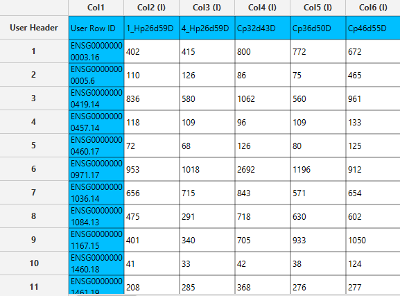
Configuration

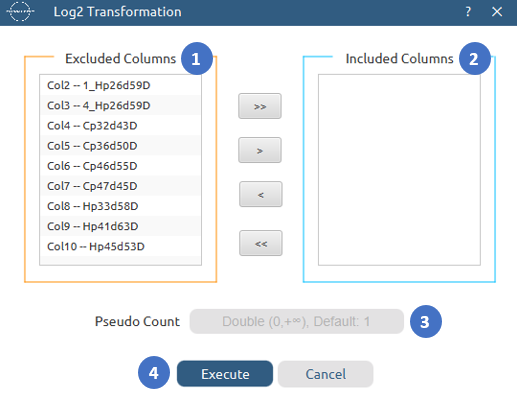
Select Data Transformation $\rightarrow$ Bio $\rightarrow$ Log2 Transformation.
Move the columns to be transformed from the Excluded Columns list [1] to the Included Columns list [2] using the arrow buttons or by double-clicking.
Set the Pseudo Count [3] to the desired additive constant.
Click the Execute button [4] to apply the transformation.

Output

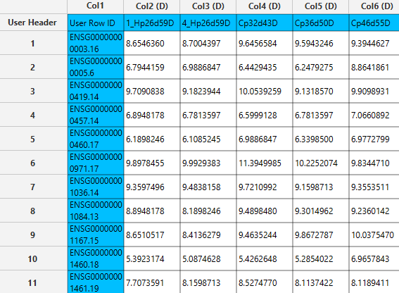
Once execution completes, the output table contains all original columns with the selected columns replaced by their log₂(x + c) values.

Log10 Transformation

The Log10 Transformation applies the element-wise function

\[f(x) = \log_{10}(x + c)\]

where c is a user-defined pseudo-count (default 1). The pseudo-count is added before the logarithm to prevent log₁₀(0) = −∞ for zero-count values and to handle near-zero measurements gracefully. Log10 is preferred over Log2 when data spans several orders of magnitude (e.g. raw fluorescence intensities, proteomics abundances) or when decade-based scales are more interpretable and comparable with reference ranges in clinical or proteomics settings.

The transformation is applied only to the columns explicitly moved to the Included Columns list; all other columns are passed through to the output unchanged.

Pre-validation

Use the Log10 Transformation biotransformation function by browsing in the top ribbon:

Data Transformation $\rightarrow$ Bio $\rightarrow$ Log10 Transformation

Input

Configuration

Excluded Columns	Lists all numerical columns available for transformation that have not yet been selected.
Included Columns	Lists the columns that will be transformed.
Pseudo Count	Specify a positive value (0, +∞) added to each selected cell before the logarithm is taken. The default value of 1 ensures that zero counts map to log₁₀(1) = 0 rather than −∞.

Output

The output table has the same dimensions as the input. Columns in the Included Columns list are replaced by their log₁₀(x + c) values; all remaining columns are copied as-is. Column headers and row IDs are preserved.

Example

Input

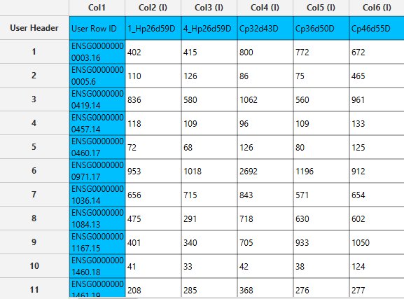
In the left-hand spreadsheet of the tab import the data matrix. Columns intended for transformation must be free of missing values.

Configuration

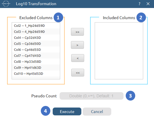
Select Data Transformation $\rightarrow$ Bio $\rightarrow$ Log10 Transformation.
Move the columns to be transformed from the Excluded Columns list [1] to the Included Columns list [2] using the arrow buttons or by double-clicking.
Set the Pseudo Count [3] to the desired additive constant.
Click the Execute button [4] to apply the transformation.

Output

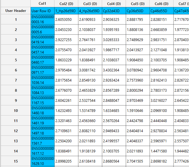
Once execution completes, the output table contains all original columns with the selected columns replaced by their log₁₀(x + c) values.

VST

The Variance Stabilising Transformation (VST) is a DESeq-based method that transforms raw RNA-Seq count data into approximately homoskedastic values — values whose variance is roughly constant across the range of means. Raw counts exhibit mean-dependent variance (low-count genes are dominated by Poisson noise; high-count genes by overdispersion), which distorts distance-based analyses such as PCA and clustering. VST removes this dependency by applying a closed-form transformation derived from a fitted negative binomial mean–dispersion model. ³

VST estimates size factors and a parametric mean–dispersion curve from the input data before transforming. VST output values are on an arbitrary variance-stabilised scale suitable for exploratory analysis but not for fold-change reporting. ⁴

Input grid layout

The input spreadsheet is organised as samples in rows, genes (count columns) in columns, with optional metadata columns (factors, covariates) alongside:

gene1 | gene2 | … | condition | batch
------+-------+---+-----------+------
 12   |  340  | … | treated   |  A      ← sample 1
  8   |  120  | … | control   |  B      ← sample 2

Columns assigned as Factors or Covariates are used to build the design matrix; all remaining numerical columns are treated as gene count columns and transformed.

Algorithm

The fit proceeds in the following steps:

Step 1 — Size factor estimation. Each sample’s size factor is estimated from the ratio of each gene count to the geometric mean across samples, taking the median across genes (DESeq median-of-ratios method).

Step 2 — Normalisation. Counts are divided by their sample size factors to obtain normalised values q[g][s].

Step 3 — Gene-wise dispersion estimation. For each gene, initial dispersion estimates are derived from the normalised counts (moments and rough GLM estimators), per-gene fitted means are obtained by fitting a negative binomial GLM to the count data under the specified design, and dispersions are then refined by optimising the Cox-Reid adjusted log-profile likelihood. The result is a per-gene dispersion $\hat{\alpha}$ that captures the mean-dependent overdispersion of the data.

Step 4 — Parametric mean–dispersion curve. A two-parameter curve

\[\hat{\alpha}(\mu) = a_0 + \frac{a_1}{\mu}\]

is fitted to the (mean, dispersion) pairs by iteratively re-fitting a Gamma GLM with identity link.

The fitted parameters a₀ (asymptotic dispersion) and a₁ (extra-Poisson dispersion coefficient) are stored and reported after execution.

Step 5 — Closed-form VST. Using the fitted curve parameters and the normalised counts q[g][s], the VST value is:

\[\text{vst}_{g,s} = \log_2\!\left(\frac{1 + a_1 + 2 a_0 q_{g,s} + 2\sqrt{a_0 q_{g,s}\left(1 + a_1 + a_0 q_{g,s}\right)}}{4 a_0}\right)\]

This is the closed-form antiderivative of 1/SD(x) under the negative binomial variance model Var(x) = μ + a₀μ² + a₁μ, evaluated at q[g][s]. q[g][s] denotes the variance-stabilized expression value obtained by applying the VST to gene (g) in sample (s).⁵

Use the VST biotransformation function by browsing in the top ribbon:

Data Transformation $\rightarrow$ Bio $\rightarrow$ VST

Input

The input spreadsheet must have samples as rows and gene count columns as numerical columns, with at least 2 samples and at least 1 gene count column. Optional metadata columns (factors, covariates) may be present alongside the count columns. Count values must be non-negative; negative values will abort execution. Missing values are not permitted in count columns.

Configuration

Excluded Columns	Lists all input columns not yet assigned as a Factor or Covariate. All unassigned numerical columns will be treated as gene count columns and transformed.
Factors	Categorical metadata columns that define experimental groups (e.g. condition, treatment). At least one factor or covariate is required unless intercept-only mode is used. Reference levels for each factor can be specified via the `Specify Reference Levels` button.
Specify Reference Levels	Opens a sub-dialog to set the reference level for each factor. The reference level determines which group is used as the baseline in the design matrix.
Covariates	Continuous numerical metadata columns to include in the design (e.g. batch scores, library size covariates). Covariate columns must be numerical; non-numerical columns are rejected at validation.
Formula Type	Controls how the design formula is constructed: - `Main Effects`: all assigned factors and covariates are included as additive main effects. - `Full Factorial`: all main effects and their interactions are included. - `Custom`: a formula is entered manually via the `Specify Custom Model Formula` button.
Specify Custom Model Formula	Opens a formula editor (active only when Custom formula type is selected). The formula must reference the assigned factor and covariate column names.
Include Intercept	When checked (default), the design matrix includes an intercept column and factors are encoded using reference contrasts. When unchecked, the formula is specified without an intercept, resulting in one indicator column per factor level and no synthetic intercept — equivalent to a cell-means parameterisation. Unchecking requires at least one factor or covariate to be assigned.

Output

The output table has the same dimensions and column order as the input. Gene count columns are replaced by their VST-transformed values; metadata columns (factors, covariates) are copied verbatim. Column headers and row IDs are preserved.

Example

Input

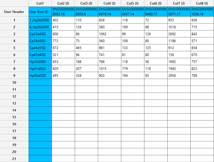
In the left-hand spreadsheet of the tab import the count matrix with samples as rows and genes as columns. Metadata columns (condition, batch, etc.) may be present alongside the count columns.

Configuration

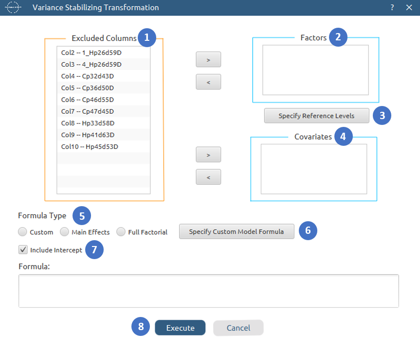
Select Data Transformation $\rightarrow$ Bio $\rightarrow$ VST.
Move any metadata columns from the Excluded Columns list [1] to the Factors [2] or Covariates [4] lists using the arrow buttons. Count columns remain in Excluded Columns and are transformed automatically.
If factors are assigned, optionally click Specify Reference Levels [3] to set the baseline level for each factor.
Select the Formula Type [5] (Main Effects, Full Factorial, or Custom). For Custom, click Specify Custom Model Formula [6] to enter the formula.
Check or uncheck Include Intercept [7] as appropriate for the experimental design.
Click the Execute button [8] to run the transformation.

Output

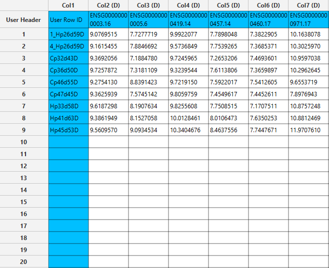
Once execution completes, the output table contains all original columns with the gene count columns replaced by their VST-transformed values. Metadata columns are copied unchanged.

RLog

The Regularised Logarithm (rlog) is a DESeq-based transformation that maps raw RNA-Seq counts to a log₂-scale representation while shrinking sample-to-sample variation for genes with low counts toward their row mean. Unlike a plain log transformation, rlog applies gene-specific shrinkage: genes with high and consistent counts across samples are transformed similarly to an ordinary log₂, while genes with low or highly variable counts are pulled toward zero fold-change relative to the average expression. This makes rlog particularly robust for small datasets where variance estimation is unstable. ³

RLog estimates size factors and a parametric mean–dispersion curve from the input data, then solves a penalised regression (ridge-regularised NB-GLM) per gene to obtain the shrunken log₂ values. The output is on an approximate log₂ scale but is not directly interpretable as log₂(count); it is suitable for exploratory analysis but not for fold-change reporting. ⁴

Input grid layout

Samples in rows, genes as numerical columns, optional metadata columns (factors, covariates) alongside:

gene1 | gene2 | … | condition | batch
------+-------+---+-----------+------
 12   |  340  | … | treated   |  A      ← sample 1
  8   |  120  | … | control   |  B      ← sample 2

Algorithm

Steps 1–2 — Size factor estimation and normalisation. Size factors are estimated by the median-of-ratios method and used to normalise counts to q[g][s] (identical to VST).

Step 3 — Gene-wise dispersion estimation. Initial dispersions are derived from normalised counts, per-gene fitted means are obtained from a negative binomial GLM, and dispersions are refined by optimising the Cox-Reid adjusted log-profile likelihood. The result is a per-gene dispersion $\hat{\alpha}$.

Step 4 — Parametric mean–dispersion trend. A two-parameter curve α̂(μ) = a₀ + a₁/μ is fitted to the (mean, dispersion) pairs by iterative Gamma GLM. The trend-smoothed dispersion at each gene’s mean expression is used as the prior for the shrinkage step.

Step 5 — Regularised shrinkage and final values. A gene-specific prior variance is estimated from the weighted spread of log-fold changes across samples, and used as a ridge penalty in a per-gene regularised negative binomial GLM. The resulting shrunken coefficients, converted to log₂ scale, form the final rlog matrix: one value per gene per sample where sample-to-sample variation has been pulled toward zero according to the strength of the prior.

Use the RLog biotransformation function by browsing in the top ribbon:

Data Transformation $\rightarrow$ Bio $\rightarrow$ RLog

Input

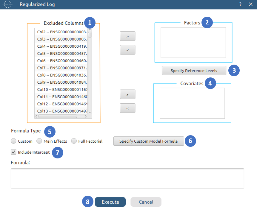
The configuration panel is identical to VST:

Excluded Columns	Lists all input columns not yet assigned as a Factor or Covariate. All unassigned numerical columns will be treated as gene count columns and transformed.
Factors	Categorical metadata columns that define experimental groups (e.g. condition, treatment). At least one factor or covariate is required unless intercept-only mode is used. Reference levels for each factor can be specified via the `Specify Reference Levels` button.
Specify Reference Levels	Opens a sub-dialog to set the reference level for each factor.
Covariates	Continuous numerical metadata columns to include in the design. Covariate columns must be numerical; non-numerical columns are rejected at validation.
Formula Type	Controls how the design formula is constructed: - `Main Effects`: all assigned factors and covariates as additive main effects. - `Full Factorial`: all main effects and their interactions. - `Custom`: a formula entered manually via the `Specify Custom Model Formula` button.
Specify Custom Model Formula	Opens a formula editor (active only when Custom formula type is selected).
Include Intercept	When checked (default), the design matrix includes an intercept column and factors are encoded using reference contrasts. When unchecked, the formula is specified without an intercept, resulting in one indicator column per factor level and no synthetic intercept — equivalent to a cell-means parameterisation. Unchecking requires at least one factor or covariate to be assigned.

Output

The output table has the same dimensions and column order as the input. Gene count columns are replaced by their rlog-transformed values; metadata columns (factors, covariates) are copied verbatim. Column headers and row IDs are preserved.

Example

Input

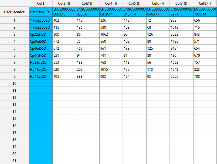
In the left-hand spreadsheet of the tab import the count matrix with samples as rows and genes as columns. Metadata columns may be present alongside the count columns.

Configuration

Select Data Transformation $\rightarrow$ Bio $\rightarrow$ RLog.
Move any metadata columns from the Excluded Columns list [1] to the Factors [2] or Covariates [4] lists. Count columns remain in Excluded Columns and are transformed automatically.
If factors are assigned, optionally click Specify Reference Levels [3] to set the baseline level for each factor.
Select the Formula Type [5] and, for Custom, click Specify Custom Model Formula [6].
Check or uncheck Include Intercept [7] as appropriate.
Click the Execute button [8] to run the transformation.

Output

Once execution completes, the output table contains all original columns with the gene count columns replaced by their rlog-transformed values. Metadata columns are copied unchanged.

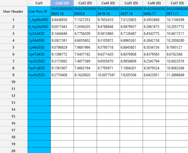
DESeq

DESeq is a full differential expression pipeline for RNA-Seq count data. It models raw counts with a negative binomial distribution, estimates per-gene dispersions using an empirical Bayes shrinkage procedure, fits a generalised linear model under a user-specified design, and tests for differential expression using either a Wald test or a likelihood ratio test (LRT). The output is a per-gene results table with fold changes, standard errors, test statistics, p-values, and Benjamini–Hochberg-adjusted p-values. ³

Input grid layout

Samples in rows, genes as numerical columns, with required metadata columns (factors, covariates) alongside:

gene1 | gene2 | … | condition | batch
------+-------+---+-----------+------
 12   |  340  | … | treated   |  A      ← sample 1
  8   |  120  | … | control   |  B      ← sample 2

All unassigned numerical columns are treated as gene count columns. At least one factor or covariate must be assigned.

Algorithm

Step 1 — Design matrix construction. The user-specified factors, covariates, reference levels, and formula are encoded into a design matrix. With Include Intercept checked, the design matrix includes an intercept column and factors are encoded using reference contrasts. With Include Intercept unchecked, the model is parameterised without an intercept; the first factor is represented by separate indicator columns for its levels, while additional factors are encoded using contrasts as needed to maintain a full-rank design matrix. For LRT, the reduced model is always constructed using reference contrasts, regardless of the full model’s intercept setting, ensuring that the reduced model is nested within the full model. ⁴

Step 2 — Size factor estimation and normalisation. Size factors are estimated by the median-of-ratios method (DESeq standard). Each gene’s count in each sample is divided by its size factor to obtain normalised counts.

Steps 3— Dispersion estimation. Per-gene dispersions are first estimated from the count data using moment-based and rough GLM estimates, followed by fitting a parametric mean–dispersion trend of the form a₀ + a₁/μ. Unlike VST, which uses the fitted mean–dispersion trend directly for the transformation, DESeq further regularises the gene-wise dispersion estimates using empirical-Bayes MAP shrinkage toward this trend. In this step, each gene’s individual dispersion estimate is combined with the overall mean–dispersion relationship estimated from all genes: estimates with limited statistical support are pulled more strongly toward the trend, whereas well-supported estimates are affected less. The MAP estimate corresponds to the dispersion value that maximises the resulting posterior probability. The final dispersion for each gene is typically the MAP estimate, unless the gene-wise estimate is identified as a dispersion outlier, in which case the original gene-wise estimate is retained.

Step 4 — NB-GLM fit (full model). A negative binomial GLM is fitted per gene under the full design matrix using IRLS (ridge-penalised, tolerance 10⁻⁸, maximum 100 iterations). The fitted coefficients (β̂) and their standard errors are used for fold-change reporting and Wald testing.

Step 5a — Wald test (when Test Type = Wald)

For each gene, the Wald statistic for the selected coefficient is:

\[W_g = \frac{\hat{\beta}_{g,k}}{\widehat{\mathrm{SE}}(\hat{\beta}_{g,k})}\]

A two-sided p-value is computed from the standard normal distribution. Log₂ fold changes and standard errors are reported for the selected coefficient.

Step 5b — Likelihood ratio test (when Test Type = LRT)

An additional NB-GLM is fitted per gene under the reduced model (the full formula minus the terms excluded by the user). The LRT statistic is:

\[\Lambda_g = 2\,(\ell_{\text{full}} - \ell_{\text{reduced}})\]

which follows a chi-squared distribution with df = p_full − p_reduced degrees of freedom. Log₂ fold changes and standard errors from the full model are still reported for the selected coefficient to support downstream visualisation (volcano plots, MA plots).

Step 6 — Multiple testing correction. P-values are adjusted across all genes using the Benjamini–Hochberg procedure (FDR control). Genes with a base mean of zero or with NA p-values (Cook’s outliers) are excluded from adjustment and receive NA in the padj column. ⁶

Use the DESeq biotransformation function by browsing in the top ribbon:

Data Transformation $\rightarrow$ Bio $\rightarrow$ DESeq

Input

The input spreadsheet must have samples as rows and gene count columns as numerical columns, with at least 2 samples. At least one factor column must be assigned. Count values must be non-negative integers; negative values will abort execution. Missing values are not permitted in count columns.

Configuration

Excluded Columns	Lists all input columns not yet assigned as a Factor or Covariate. All unassigned numerical columns are treated as gene count columns.
Factors	Categorical metadata columns defining experimental groups (e.g. condition, treatment). At least one factor is required. Reference levels for each factor can be set via the `Specify Reference Levels` button.
Specify Reference Levels	Opens a sub-dialog to set the baseline level for each factor. The reference level determines which group is the denominator in fold-change calculations.
Covariates	Continuous numerical metadata columns included in the design (e.g. batch scores). Covariate columns must be numerical.
Formula Type	Controls how the design formula is constructed: - `Main Effects`: all assigned factors and covariates as additive main effects. - `Full Factorial`: all main effects and their pairwise interactions. - `Custom`: a formula entered manually via the `Specify Custom Model Formula` button.
Specify Custom Model Formula	Opens a formula editor (active only when Custom formula type is selected).
Include Intercept	When checked (default), factors are encoded as reference contrasts with an intercept. When unchecked, a cell-means parameterisation is used. Unchecking requires at least one factor or covariate.
Test Type	Choose the statistical test: - `Wald`: tests a single selected coefficient using the Wald z-statistic. Suitable for simple two-group or multi-factor contrasts. - `LRT`: compares the full model against a reduced model using a likelihood ratio test. Suitable for testing the overall contribution of a factor or set of terms.
Output Coefficient	Select the encoded coefficient to test and report. The combo box is populated after factors and formula are specified, listing one entry per design matrix column. If LRT is selected, only coefficients that are present in both the full and reduced models are included in the output options.
Reduced Terms	(LRT only) A checklist of all terms in the full formula. Check any term to exclude it from the reduced model. Interaction terms are automatically excluded when a constituent main effect is excluded. A preview of the reduced formula is shown below the checklist.

Output

The output table contains one row per gene with the following columns:

Column	Content
Row ID	Gene name (taken from the count column headers).
`baseMean`	Mean of normalised counts across all samples.
`log2FoldChange`	Log₂ fold change for the selected coefficient.
`lfcSE`	Standard error of the log₂ fold change.
`stat`	Wald z-score (Wald test) or likelihood ratio statistic (LRT).
`pvalue`	Raw p-value. NA for genes with zero base mean.
`padj`	Benjamini–Hochberg-adjusted p-value.

Example

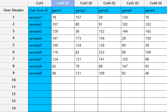
Input

In the left-hand spreadsheet of the tab import the count matrix with samples as rows and genes as columns. Metadata columns (condition, batch, etc.), if exist, must be present alongside the count columns.

Configuration

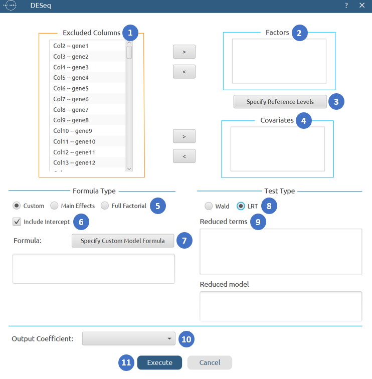
Select Data Transformation $\rightarrow$ Bio $\rightarrow$ DESeq.
Move metadata columns from the Excluded Columns list [1] to the Factors [2] or Covariates [4] lists. Count columns remain in Excluded Columns and are tested automatically.
Click Specify Reference Levels [3] to set the baseline level for each factor.
Select the Formula Type [5] and, for Custom, check or uncheck Include Intercept [6] as appropriate, click Specify Custom Model Formula [7].
Select the Test Type [8]: Wald or LRT.
For LRT, check also the terms to exclude from the Reduced Terms list [9].
Select the Output Coefficient [10] to test.
Click the Execute button [11] to run the pipeline.

Output

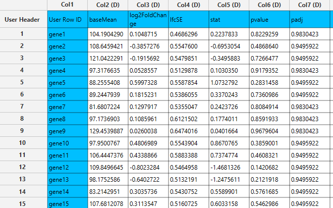
Once execution completes, the output table lists one row per gene with base mean, log₂ fold change, standard error, test statistic, raw p-value, and adjusted p-value.

Post Process DESeq

The Post Process DESeq node provides downstream analyses and data extractions that operate on the results of an upstream DESeq node without re-running the algorithm. It reads the result arrays stored in the DESeq configuration (normalised counts, size factors, dispersions, Cook’s distances, fold changes, p-values) and applies one of two top-level modes: Output Option or Post Process Option. ³

Use the Post Process DESeq bio function by browsing in the top ribbon:

Data Transformation $\rightarrow$ Bio $\rightarrow$ Post Process DESeq

The node must be placed downstream of an executed DESeq node in the same workflow. It is invalidated automatically whenever the upstream DESeq node is re-executed.

Input

The input spreadsheet is ignored, regardless of which dataset is imported. All required data are retrieved directly from the selected previously executed DESeq node.

Configuration

DESeq Analysis	Select the upstream DESeq node whose stored results this node will use.
Operation	Choose between `Output Option` (retrieve a stored array) and `Post-Processing Option` (run a downstream analysis).

Output Option — retrieves one of three arrays stored by the upstream DESeq node and writes it as a table:

Option	Output
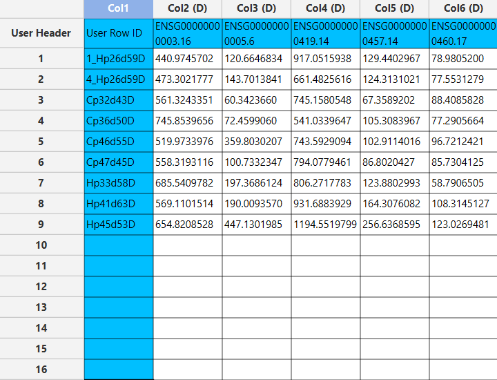
`Normalized counts`	A table with samples as rows and genes as columns, containing each gene’s count divided by the sample’s size factor. Row IDs are sample names.
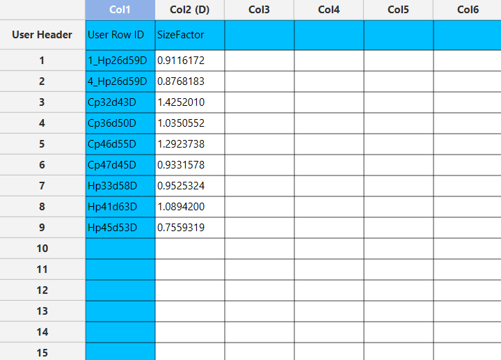
`Size factors`	A single-column table listing each sample’s size factor. Row IDs are sample names.
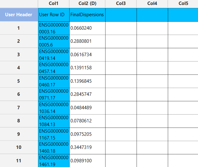
`Final dispersions`	A single-column table listing the final per-gene dispersion estimate (after MAP shrinkage). Row IDs are gene names.

Post-Processing Option — runs one of four downstream analyses:

Outliers’ check using Cook’s distance
Filters out genes whose maximum Cook’s distance across samples exceeds a threshold, returning the raw count matrix of the surviving genes only.⁷

Cook’s Distance sub-configuration:

Parameter	Description
Default Cutoff	Uses the default cutoff — the 99th percentile of the F(p, m−p) distribution, where p = number of model coefficients and m = number of samples.
Custom Cutoff	Specify a user-supplied positive value. Default: -

Replace Outliers
Replaces raw counts flagged as Cook’s distance outliers with a trimmed-mean-based estimate before returning the modified count matrix. The output is a count matrix (samples × genes) with replaced values.

The replacement procedure is:

A sample is replaceable when its design-matrix row is shared by at least minReplicates other samples (i.e. its experimental group has sufficient replicates).
The trimmed base mean is computed per gene by sorting normalised counts across samples, removing trim fraction from each tail, and averaging the remainder.
The replacement count for sample s is: round(trimmed base mean × size factor[s]).
For every (gene, sample) pair where Cook’s distance exceeds the cutoff and the sample is replaceable, the raw count is replaced with the replacement count.

Replace Outliers sub-configuration:

Parameter	Description
Trim	Fraction to trim from each tail of normalised counts when computing the trimmed base mean. Range [0, 0.5]. Default: 0.2.
Min Replicates	Minimum number of samples a group must contain for outlier replacement to be applied to that group. Must be ≥ 3 and < number of samples. Default: 7.
Default Cutoff	Uses the default cutoff — the 99th percentile of the F(p, m−p) distribution, where p = number of model coefficients and m = number of samples.
Custom Cutoff	Specify a user-supplied positive value. Default: -

LFC shrinkage
Applies posterior shrinkage to the log₂ fold changes estimated by the upstream DESeq node, reducing noise for low-count or high-dispersion genes. Three shrinkage methods are available:

Method	Description
`normal`	Estimates a per-coefficient prior variance from the weighted spread of observed fold changes (weighted upper quantile at the 95th percentile, weight = 1/(1/μ + α̂)), then re-runs the Wald test with this prior as a ridge penalty. The intercept receives a near-zero prior variance (10⁶). Not supported for designs with interaction terms.
`apeglm`	Fits a Cauchy prior (t-distribution with df=1) on the coefficient of interest using a negative binomial Cauchy regression (ApeglmNbinomCR). The prior scale is estimated by solving for the variance that matches the observed MLE spread. All other coefficients are not shrunk (assigned a wide Cauchy prior with scale 15).
`ashr`	Uses the adaptive shrinkage (ashr) framework: a mixture of normals prior is fitted to the MLE fold changes and their standard errors, and posterior means are computed. The mixture weights are estimated by maximum likelihood (mixSQP active-set solver with EM warm-start).

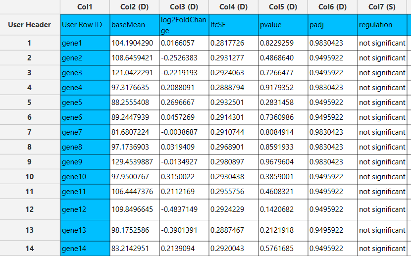
The output table has the same columns as the DESeq results table (baseMean, log2FoldChange, lfcSE, stat, pvalue, padj) with fold changes and standard errors replaced by the shrunken estimates.

LFC Shrinkage sub-configuration:

Parameter	Description
Shrinkage Type	Select the shrinkage method: `normal`, `apeglm`, or `ashr`. Default: normal.
Regulation Analysis	Optional. When enabled, appends a `regulation` column to the output classifying each gene as upregulated, downregulated, or not significant based on the shrunken fold change and a significance threshold (see Regulation Analysis below).

Regulation analysis
Classifies each gene as upregulated, downregulated, or not significant based on its fold change and a significance threshold applied to either the raw p-value or the adjusted p-value.⁶

Classification rules:

upregulated: selected p-value < p-threshold and log₂FoldChange > LFC threshold
downregulated: selected p-value < p-threshold and log₂FoldChange < −LFC threshold
not significant: otherwise (including genes with NA p-values)

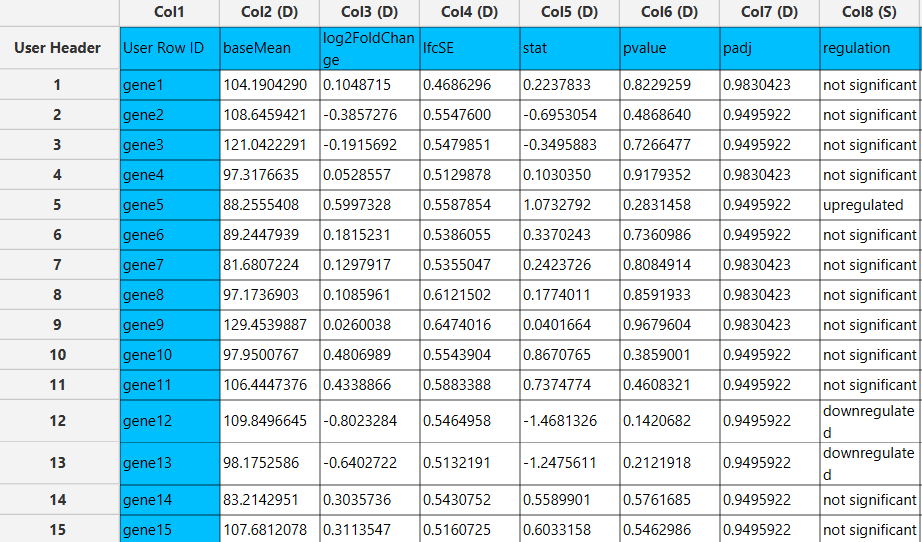
The output replicates the DESeq results table with an additional regulation column.

Regulation Analysis sub-configuration:

Parameter	Description
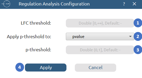
LFC Threshold	Minimum absolute log₂ fold change required for a gene to be classified as regulated. Range [0, +∞). Default: 0.0 (any direction counts).
Apply p-threshold to	Choose whether to apply the threshold to `pvalue` (raw) or `padj` (Benjamini–Hochberg adjusted). Default: pvalue.
p-threshold	Significance threshold applied to the selected p-value type. Range (0, 1). Default: 0.05.

Output

Output structure depends on the selected mode and operation:

Mode / Operation	Row IDs	Columns
Normalized counts	Sample names	One column per gene with normalised count values.
Size factors	Sample names	`SizeFactor`
Final dispersions	Gene names	`FinalDispersion`
Outliers’ check	Sample names	Genes whose maximum Cook’s distance across samples doesn’t exceed threshold
Replace outliers	Sample names	One column per gene with (possibly replaced) integer counts.
LFC shrinkage	Gene names	baseMean, log2FoldChange (shrunken), lfcSE (shrunken), stat, pvalue, padj [, regulation]
Regulation analysis	Gene names	baseMean, log2FoldChange, lfcSE, stat, pvalue, padj, regulation

Example

Input

The Post Process DESeq node does not take a spreadsheet input directly. It reads from the stored results of an upstream DESeq node. Ensure the DESeq node has been executed before opening this configuration.

Configuration

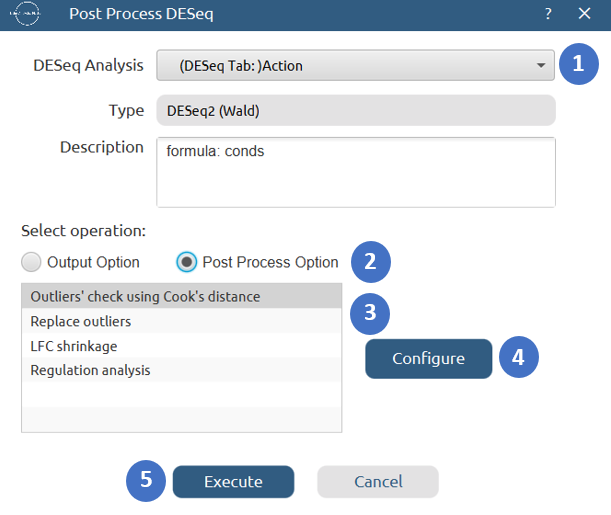
Select Data Transformation $\rightarrow$ Bio $\rightarrow$ Post Process DESeq.
Select the upstream DESeq Analysis node [1] whose results to use.
Choose the Operation [2]: Output Option or Post-Processing Operation.
For Output Option, select from listview the desired Output [3] (Normalized counts, Size factors, or Final dispersions), for Post-Processing Option, select from refreshed listview the desired Function [3] and click the Configure button [4] to set its parameters.
Click the Execute button [5] to produce the output.

Output Option

This mode does not require a configuration window. The desired output (normalized counts, size factors, final dispersions) is generated directly based on the option selected from the list view.

Post Process Option

Outliers’ check using Cook’s distance Configuration

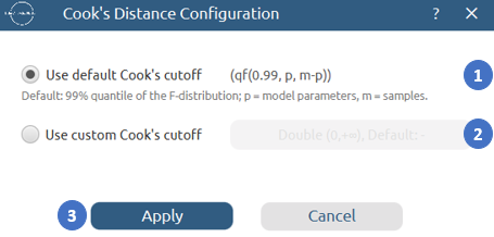
Select Use default Cook's cutoff [1] or Use custom Cook's cutoff [2] and enter a value.
Click Apply [3] in order the parametres to be saved.

Replace outliers Configuration

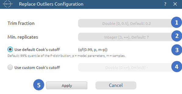
Optionally set Trim fraction [1] and Min. replicates [2]. Leave blank to use defaults.
Select Use default Cook's cutoff [3] or Use custom Cook's cutoff [4] and enter a value.
Click Apply [5], in order the parametres to be saved.

LFC shrinkage Configuration

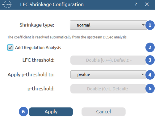
Select the Shrinkage type [1] (normal, apeglm, or ashr).
Optionally check Add Regulation Analysis [2] and set the LFC threshold [3], Apply p-threshold to [4], and p-threshold [5].
Click Apply [6], in order the parametres to be saved.

Regulation Analysis Configuration

Set the LFC threshold [1], select Apply p-threshold to [2] (pvalue or padj), and set the p-threshold [3].
Click Apply [4], in order the parametres to be saved.

Output

The output is generated according to the selected post-processing option and is presented as a table containing the corresponding results derived from the upstream DESeq analysis.

Output Option

The available outputs, depending on the option selected by the user, are:

Normalized Counts

Once execution completes, the output will contain the normalized count matrix generated from the selected upstream DESeq node.

Size Factors

Once execution completes, the output will contain the size factors estimated by the selected upstream DESeq node.

Final Dispersions

Once execution completes, the output will contain the final dispersions estimated by the selected upstream DESeq node.

Post Process Option

The available outputs, depending on the option selected by the user, are:

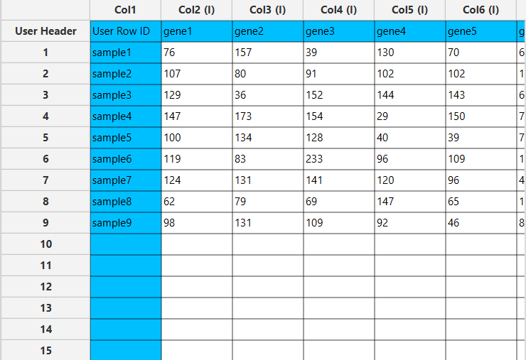
Outliers’ check using Cook’s distance Output

Once execution completes, the output contains the raw count matrix with Cook’s distance outlier genes removed. Surviving genes appear as columns; samples appear as rows.

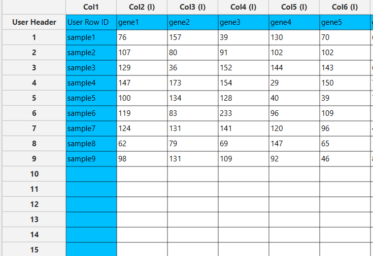
Replace Outliers Output

Once execution completes, the output contains the count matrix with outlier values replaced.

LFC Shrinkage Output

Once execution completes, the output contains the shrunken fold changes and, if enabled, the regulation classification.

Regulation Analysis Output

Once execution completes, the output appends a regulation column classifying each gene.

Normalize Between Arrays

Normalize Between Arrays (NBA) aligns the distribution of values across multiple columns (arrays) so that systematic differences in scale or location between columns are removed. It is a column-wise normalisation: each column is rescaled or adjusted relative to the others so that cross-column comparisons become meaningful. The method is derived from microarray preprocessing practice and is applicable to any tabular data where columns represent independently measured samples.¹

Three normalisation methods are available:

Quantile — forces every included column to have exactly the same empirical distribution. For each column the values are ranked, sorted, and replaced by the row means of the rank-sorted matrix. Ties receive the average of the corresponding rank-mean values (linear interpolation). Columns with missing values are handled by interpolating their sorted values onto the common quantile grid before averaging, and back-interpolating the result onto the observed ranks.⁸

Scale — scales each column by its median relative to the geometric mean of all column medians. For each included column j the scaling factor is:

\[s_j = \exp\!\left(\log\, \mathrm{median}(x_j) - \frac{1}{C}\sum_{k=1}^{C}\log\, \mathrm{median}(x_k)\right)\]

Every value in column j is divided by s_j, so that all column medians are equalised on the geometric-mean scale.

Cyclic Loess — applies 3 iterations of pairwise loess normalisation in a cyclic fashion. In each iteration, for every column i the column values are regressed against the current row means using a locally weighted scatterplot smoother (LOWESS, span = 0.7, 3 robustness iterations using bisquare weights), and the fitted loess curve is subtracted from the column. Repeating this cycle brings all columns into alignment with their common mean trend.

Use the Normalize Between Arrays function by browsing in the top ribbon:

Data Transformation $\rightarrow$ Bio $\rightarrow$ Normalize Between Arrays

Input

The data input should consist of numerical instances without missing values in the columns to be normalised. At least 2 numerical columns are required. Non-numerical columns are permitted and will be passed through to the output unchanged.

Configuration

Excluded Columns	Lists all numerical columns not yet selected for normalisation.
Included Columns	Lists the columns that will be normalised together.
Method	Select the normalisation method: `Quantile`, `Scale`, or `Cyclic Loess`. Default: Quantile.

Output

The output table has the same dimensions and column order as the input. Columns in the Included Columns list are replaced by their normalised values; all other columns are copied as-is. Column headers and row IDs are preserved.

Example

Input

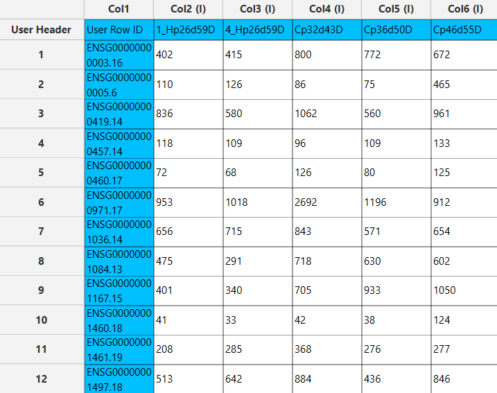
In the left-hand spreadsheet of the tab import the data matrix. Columns intended for normalisation must be numerical.

Configuration

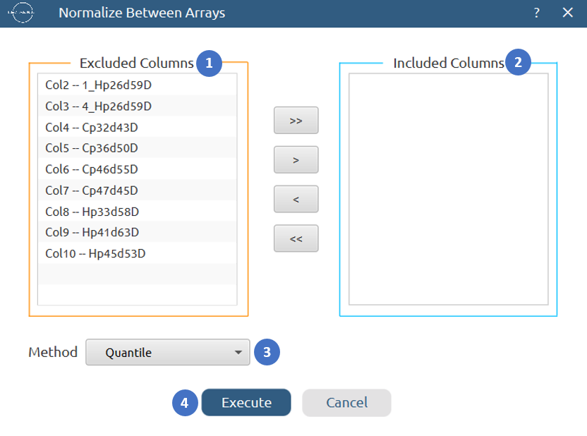
Select Data Transformation $\rightarrow$ Bio $\rightarrow$ Normalize Between Arrays.
Move the columns to normalise from the Excluded Columns list [1] to the Included Columns list [2] using the arrow buttons or by double-clicking.
Select the normalisation Method [3].
Click the Execute button [4] to run the normalisation.

Output

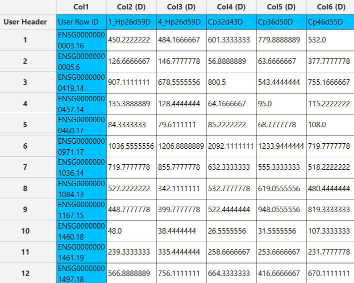
Once execution completes, the output table contains all original columns with the selected columns replaced by their normalised values.

Limma

Limma (Linear Models for Microarray and RNA-Seq Data) is a differential expression pipeline that fits a linear model to each gene’s expression values across samples and tests for differences between groups using moderated t-statistics.¹ Variance moderation via empirical Bayes borrows information across genes to stabilise per-gene variance estimates, making the method particularly powerful for experiments with small sample sizes. Limma was originally developed for microarray data and is fully applicable to any log-scale expression matrix. ⁹

Input grid layout

Samples in rows, genes (expression columns) as numerical columns, with optional metadata columns (factors, covariates) alongside:

gene1 | gene2 | … | condition | batch
------+-------+---+-----------+------
 5.2  |  8.1  | … | treated   |  A      ← sample 1
 4.9  |  7.8  | … | control   |  B      ← sample 2

Columns assigned as Factors or Covariates are used to build the design matrix; all remaining numerical columns are treated as gene expression columns and tested. Unlike DESeq, limma expects pre-normalised, log-scale input (e.g. log₂-CPM, rlog, or VST values). Raw counts should be transformed before using this node.

Algorithm

Step 1 — Design matrix construction. Identical to DESeq: the user-specified factors, covariates, reference levels, and formula are encoded into a design matrix. With Include Intercept checked, the design matrix includes an intercept column and factors are encoded using reference contrasts. With Include Intercept unchecked, the model is parameterised without an intercept.

Step 2 — Linear model fitting. A linear model is fitted per gene by regressing each gene’s expression vector (length S) onto the design matrix using one of two methods:

Least Squares (default): ordinary least squares (OLS) — computes $\hat{\beta} = (X^T X)^{-1} X^T y$ using QR decomposition. Residual variance $\hat{\sigma}^2$ is estimated from the residual sum of squares with $S - p$ degrees of freedom.
Robust Regression: M-estimation with Huber weights, iterating until convergence to downweight outlier samples. The effective degrees of freedom are adjusted for the sum of weights.

Step 3 — Empirical Bayes variance moderation (when Use Empirical Bayes is checked)

The per-gene residual variances $\hat{\sigma}_g^2$ are pooled across all genes by fitting a scaled inverse chi-squared prior (s₀², ν₀) to the observed variance distribution. The moderated variance for each gene is:

\[\tilde{\sigma}_g^2 = \frac{\nu_0 s_0^2 + \nu_g \hat{\sigma}_g^2}{\nu_0 + \nu_g}\]

where ν_g = S − p is the residual degrees of freedom. This shrinks extreme per-gene variances toward the global prior, replacing the noisy per-gene estimate with a stabilised one. Moderated t-statistics use ν₀ + ν_g degrees of freedom.

When Use Empirical Bayes is unchecked, ordinary t-statistics are computed directly from the OLS or robust estimates without variance borrowing.

Step 4 — Testing and output statistics. For the selected output coefficient k, the following are computed per gene:

logFC: the estimated coefficient $\hat{\beta}_k$ (log-fold change on the input scale).
AveExpr: mean expression across all samples.
t: moderated t-statistic (or ordinary t if EB is off) = $\hat{\beta}_k$/ ($\tilde{\sigma}_g$ · SE_k).
P.Value: two-tailed p-value from the t-distribution with ν₀ + ν_g degrees of freedom.
adj.P.Val: Benjamini–Hochberg-adjusted p-value across all genes.
B: log-odds that the gene is differentially expressed (B-statistic, lods), computed from the moderated F framework. Only meaningful when Use Empirical Bayes is checked.

Use the Limma biotransformation function by browsing in the top ribbon:

Data Transformation $\rightarrow$ Bio $\rightarrow$ Limma

Input

The input spreadsheet must have samples as rows and gene expression columns as numerical columns, with at least 2 complete numerical expression columns and at least 2 samples. The expression values should be on a log scale (e.g. log₂-CPM, rlog, VST). Missing values are not permitted in expression columns. Optional metadata columns (factors, covariates) may be present alongside.

Configuration

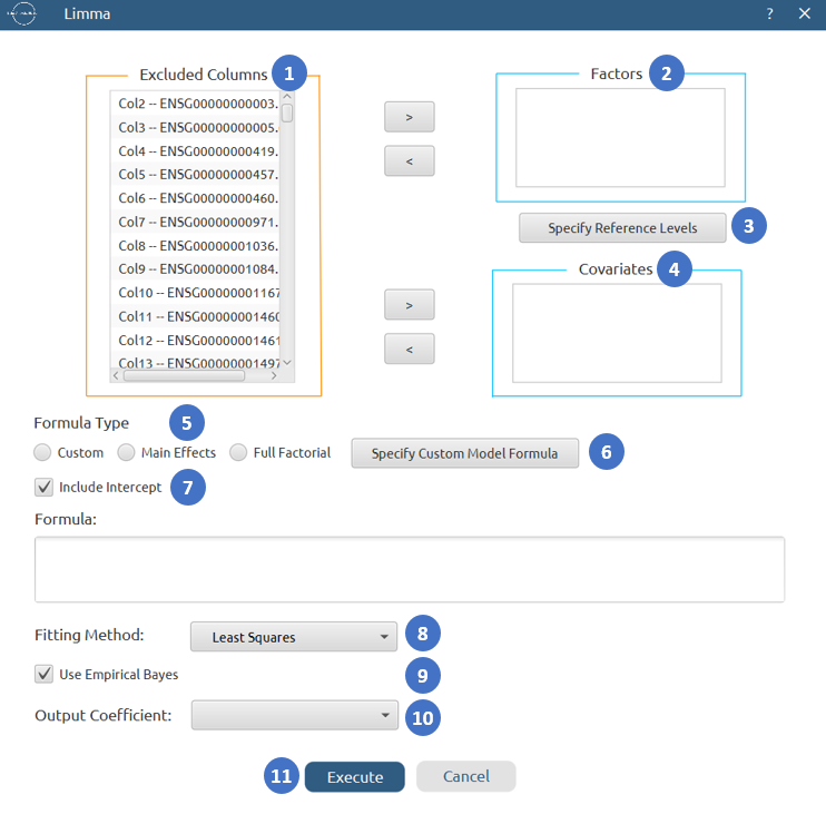
Excluded Columns	Lists all input columns not yet assigned as a Factor or Covariate. All unassigned numerical columns are treated as gene expression columns and tested.
Factors	Categorical metadata columns defining experimental groups (e.g. condition, treatment).
Specify Reference Levels	Opens a sub-dialog to set the baseline level for each factor.
Covariates	Continuous numerical metadata columns to include in the design (e.g. batch scores). Covariate columns must be numerical.
Formula Type	Controls how the design formula is constructed: - `Main Effects`: all assigned factors and covariates as additive main effects. - `Full Factorial`: all main effects and their pairwise interactions. - `Custom`: a formula entered manually via the `Specify Custom Model Formula` button.
Specify Custom Model Formula	Opens a formula editor (active only when Custom formula type is selected).
Include Intercept	When checked (default), factors are encoded as reference contrasts with an intercept. When unchecked, a cell-means parameterisation is used. Unchecking requires at least one factor or covariate.
Fitting Method	Select the linear model fitting method: - `Least Squares`: ordinary least squares via QR decomposition. - `Robust Regression`: M-estimation with Huber weights, downweighting outlier samples.
Use Empirical Bayes	When checked (default), applies empirical Bayes variance moderation across genes, producing moderated t-statistics, moderated degrees of freedom, and the B-statistic. When unchecked, ordinary per-gene t-statistics are reported and the B column is not meaningful.
Output Coefficient	Select the encoded design matrix coefficient to test and report. The combo box is populated automatically after factors and formula are specified, listing one entry per design matrix column.

Output

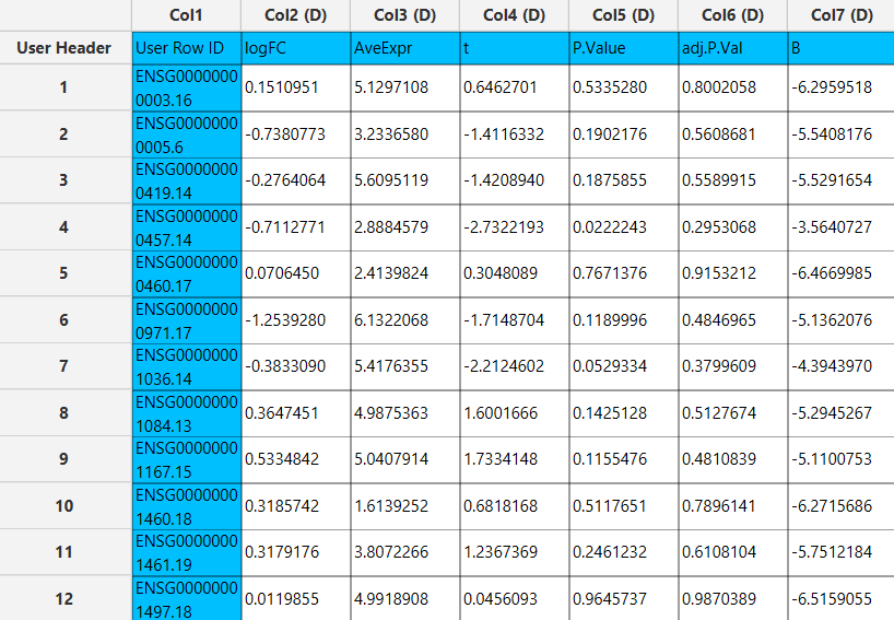
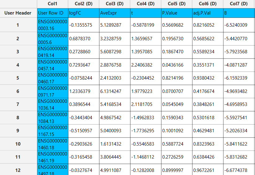
The output table contains one row per gene with the following columns:

Column	Content
Row ID	Gene name.
`logFC`	Log-fold change for the selected coefficient (β̂_k on the input scale).
`AveExpr`	Mean expression across all samples.
`t`	Moderated t-statistic (or ordinary t if empirical Bayes is off).
`P.Value`	Raw two-tailed p-value.
`adj.P.Val`	Benjamini–Hochberg-adjusted p-value.
`B`	Log-odds of differential expression (B-statistic). Meaningful only when Use Empirical Bayes is checked.

Example

Input

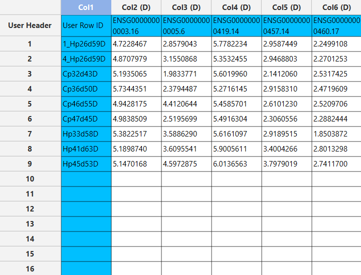
In the left-hand spreadsheet of the tab import the expression matrix with samples as rows and genes as columns. The data should be on a log scale. Metadata columns (condition, batch, etc.) must be present alongside the expression columns.

Configuration

Select Data Transformation $\rightarrow$ Bio $\rightarrow$ Limma.
Move metadata columns from the Excluded Columns list [1] to the Factors [2] or Covariates [4] lists. Expression columns remain in Excluded Columns and are tested automatically.
Optionally click Specify Reference Levels [3] to set the baseline level for each factor.
Select the Formula Type [5] (Main Effects, Full Factorial, or Custom). For Custom, click Specify Custom Model Formula [6].
Check or uncheck Include Intercept [7] as appropriate.
Select the Fitting Method [8]: Least Squares or Robust Regression.
Check or uncheck Use Empirical Bayes [9].
Select the Output Coefficient [10] to test and report.
Click the Execute button [11] to run the pipeline.

Output

Once execution completes, the output table lists one row per gene with logFC, AveExpr, t-statistic, raw p-value, adjusted p-value, and B-statistic.

Voom

Voom (variance modelling at the observation level) is a preprocessing step that bridges raw RNA-Seq count data and the limma linear modelling framework. It converts raw counts to log₂-CPM values, fits a mean-variance trend across genes, and derives per-observation precision weights that capture the heteroskedastic nature of count data. The resulting log₂-CPM matrix and weight matrix are then passed to a weighted limma fit, allowing limma’s empirical Bayes machinery — originally designed for homoskedastic microarray data — to be applied correctly to RNA-Seq counts. ¹⁰

Voom combines two operations into one node: the count-to-log₂-CPM transformation (with optional between-array normalisation) and the subsequent weighted limma differential expression test. The output is a results table identical in structure to the limma node.

Input grid layout

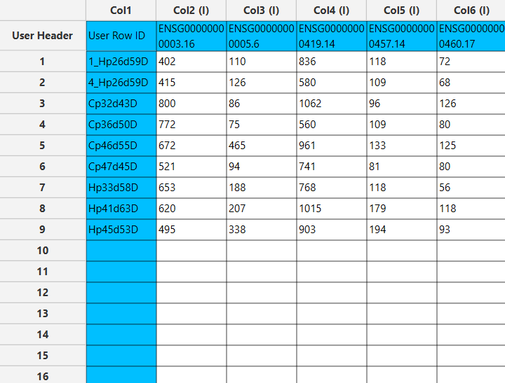
Samples in rows, genes (count columns) as numerical columns, with required metadata columns (factors, covariates) alongside. Unlike limma, voom expects raw, un-normalised integer counts as input, not log-scale expression values.

Algorithm

Step 1 — Library sizes. Each sample’s library size is computed as the column sum of all counts: lib.size[s] = Σ_g counts[g][s].

Step 2 — log₂-CPM transformation. Raw counts are converted to log₂-counts-per-million with a pseudo-count of 0.5:

\[y_{g,s} = \log_2\!\left(\frac{\text{counts}_{g,s} + 0.5}{\text{lib.size}_s + 1} \times 10^6\right)\]

Step 2b — Between-array normalisation (optional) If a normalisation method other than none is selected, normalizeBetweenArrays is applied to the log₂-CPM matrix y before the initial fit. The available methods (scale, quantile, cyclicloess) delegate to the same implementation used by the Normalize Between Arrays node.

Step 3 — Initial unweighted linear model fit. An ordinary least-squares model is fitted per gene to the log₂-CPM matrix using the specified design matrix. Residual standard deviations σ̂_g and per-gene mean expression values are computed from this initial fit.

Step 4 — Mean-variance trend (LOWESS).

For each gene, the x-coordinate is:

\[s_{x,g} = \bar{y}_g + \overline{\log_2(\mathrm{lib.size}+1)} - \log_2(10^6)\]

which approximates the log₂ count level on a library-size-adjusted scale. The y-coordinate is:

\[\sqrt{\hat{\sigma}_g}\]

A LOWESS curve is fitted to the $(s_{x,g}, \sqrt{\hat{\sigma}_g})$ pairs to estimate the overall mean-variance relationship across genes. The smoothing span is user-specified (default: 0.5), and three robustness iterations are performed to reduce the influence of outlying genes. Genes with zero counts across all samples are excluded from the fit.

Step 5 — Observation-level precision weights.

For each gene–sample pair, the fitted log-expression value from the initial linear model is converted back to the count scale using the corresponding library size. The resulting fitted count is then expressed on the log₂ scale and used to interpolate the LOWESS mean-variance trend fitted in Step 4. This provides the expected value of $\sqrt{\hat{\sigma}}$ at the fitted expression level.

The observation-level precision weight is then calculated as:

\[w_{g,s} = \frac{1}{ f(\text{fitted log-count}_{g,s})^4 }\]

where $f(\cdot)$ is the LOWESS-fitted mean-variance trend. Since the LOWESS curve models $\sqrt{\hat{\sigma}}$, raising its fitted value to the fourth power yields the corresponding variance estimate, so the resulting weight is its inverse.

These weights encode the mean-variance relationship at the observation level: observations associated with higher expected variance receive lower weights, while those associated with lower expected variance receive higher weights.

Step 6 — Weighted limma fit.

The log₂-CPM matrix and the observation-level precision weights obtained in Step 5 are used to fit the limma model. The model is fitted using the user-selected fitting method (Least Squares or Robust Regression) and the selected empirical Bayes option.

From this point onward, the analysis follows the same procedure as the standard limma node. The fitted coefficients and their standard errors are used to compute moderated t-statistics and B-statistics, and the resulting p-values are adjusted for multiple testing using the Benjamini–Hochberg procedure.

Use the Voom bio function by browsing in the top ribbon:

Data Transformation $\rightarrow$ Bio $\rightarrow$ Voom

Input

The input spreadsheet must have samples as rows and gene count columns as numerical columns, with at least 2 complete numerical count columns and at least 2 samples. Count values must be non-negative. Missing values are not permitted in count columns. At least one factor column must be assigned. Unlike the limma node, the input must be raw counts, not log-transformed values.

Configuration

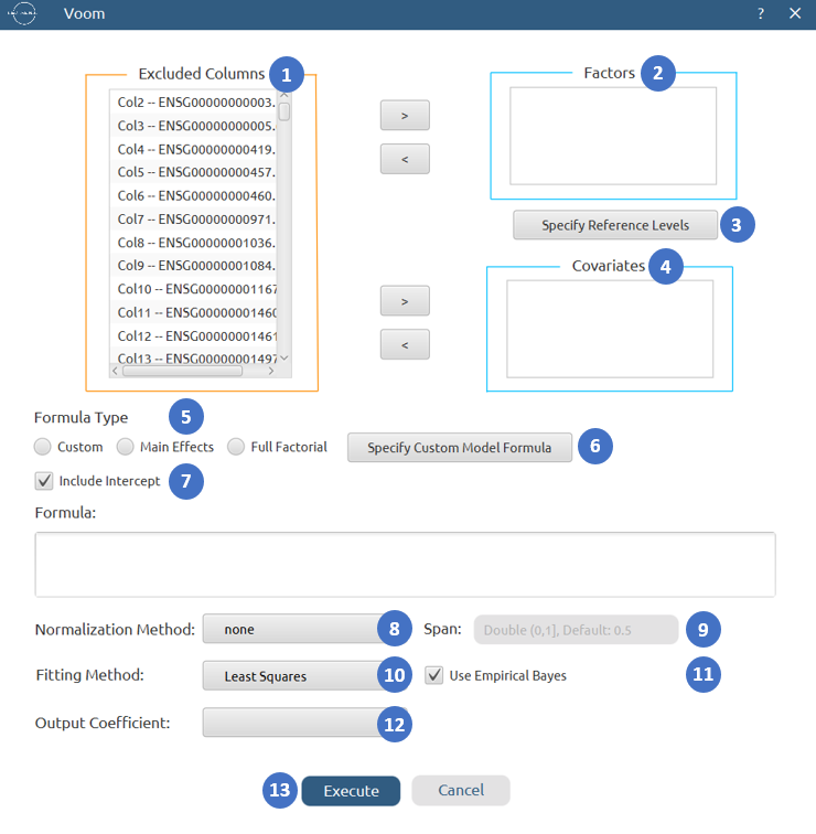
Excluded Columns	Lists all input columns not yet assigned as a Factor or Covariate. All unassigned numerical columns are treated as gene count columns.
Factors	Categorical metadata columns defining experimental groups (e.g. condition, treatment).
Specify Reference Levels	Opens a sub-dialog to set the baseline level for each factor.
Covariates	Continuous numerical metadata columns to include in the design. Must be numerical.
Formula Type	Controls how the design formula is constructed: - `Main Effects`: all assigned factors and covariates as additive main effects. - `Full Factorial`: all main effects and their pairwise interactions. - `Custom`: a formula entered manually via the `Specify Custom Model Formula` button.
Specify Custom Model Formula	Opens a formula editor (active only when Custom formula type is selected).
Include Intercept	When checked (default), factors are encoded as reference contrasts with an intercept. When unchecked, a cell-means parameterisation is used. Unchecking requires at least one factor or covariate.
Normalization Method	Between-array normalisation applied to the log₂-CPM matrix before the initial fit. Options: `none` (default), `scale`, `quantile`, `cyclicloess`. These correspond directly to the methods in the Normalize Between Arrays node.
Span	Lowess smoothing fraction for the mean-variance trend fit. Range: (0, 1]. Default: 0.5. Smaller values produce a tighter fit; larger values produce a smoother trend.
Fitting Method	`Least Squares` or `Robust Regression`. Default: Least Squares.
Use Empirical Bayes	When checked (default), applies eBayes moderation for moderated t-statistics and B-statistic.
Output Coefficient	Select the encoded design matrix coefficient to test and report.

Output

The output table is identical to the limma node — one row per gene:

Column	Content
Row ID	Gene name (taken from the count column headers).
`logFC`	Log₂ fold change for the selected coefficient.
`AveExpr`	Mean log₂-CPM expression across all samples.
`t`	Moderated t-statistic (or ordinary t if empirical Bayes is off).
`P.Value`	Raw two-tailed p-value.
`adj.P.Val`	Benjamini–Hochberg-adjusted p-value.
`B`	Log-odds of differential expression. Meaningful only when Use Empirical Bayes is checked.

Example

Input

In the left-hand spreadsheet of the tab import the raw count matrix with samples as rows and genes as columns. Metadata columns (condition, batch, etc.) must be present alongside the count columns.

Configuration

Select Data Transformation $\rightarrow$ Bio $\rightarrow$ Voom.
Move metadata columns from the Excluded Columns list [1] to the Factors [2] or Covariates [4] lists. Count columns remain in Excluded Columns.
Optionally click Specify Reference Levels [3] to set the baseline level for each factor.
Select the Formula Type [5] and, for Custom, click Specify Custom Model Formula [6].
Check or uncheck Include Intercept [7] as appropriate.
Select the Normalization Method [8] and set the Span [9] if the defaults are not appropriate.
Select the Fitting Method [10] and check or uncheck Use Empirical Bayes [11].
Select the Output Coefficient [12] to test and report.
Click the Execute button [13] to run the pipeline.

Output

Once execution completes, the output table lists one row per gene with logFC, AveExpr, t-statistic, raw p-value, adjusted p-value, and B-statistic — identical in structure to the limma output.

Tips

Log2/Log10 Transformation

The default pseudo-count of 1 is appropriate for integer count data (e.g., raw RNA-Seq counts or microarray intensities) where zero values are common. For data that is already normalised or continuous and strictly positive, a pseudo-count of 0 is mathematically valid but not permitted here — use a very small value such as 0.001 instead.
Prefer Log10 over Log2 when the data spans several orders of magnitude (e.g. fluorescence intensities from 10 to 10⁶) or when the results need to be compared against decade-based reference values in clinical or proteomics contexts.

VST/RLog

VST is recommended for datasets with many samples (n ≥ 30). For small sample sizes (n < 30), rlog is generally preferred as it applies stronger regularisation to low-count genes. RLog is recommended for datasets with few samples (n < 30). For larger datasets, VST is faster and produces comparable results.
VST output is suitable for exploratory analyses such as PCA, t-SNE, UMAP.
Rlog applies stronger shrinkage to low-count genes than VST. Genes with very low counts across all samples will be pulled close to zero on the rlog scale, effectively down-weighting them in downstream analyses

DESeq

DESeq expects raw, non-negative integer counts. Do not use TPM, FPKM, CPM, log-transformed counts, or other pre-normalised expression values as input. DESeq performs its own library-size normalisation through estimated size factors.
The reference level determines the direction of the reported log2 fold change. For a comparison treated vs. control, a positive log2 fold change indicates higher expression in the treated group and a negative value indicates lower expression.
A padj value of NA does not necessarily indicate an error. It can occur when a gene is removed by independent filtering because of very low information, or when an extreme count is identified through Cook’s distance as a potential outlier.
The Wald test is appropriate when testing a specific pairwise contrast (e.g. treated vs. control). The LRT is appropriate when testing whether a factor as a whole contributes to expression variation — for example, when a factor has more than two levels and no single contrast captures the full effect.
For the LRT, the reduced model must be nested within the full model. Excluding a main effect automatically excludes all interaction terms containing it.
The padj column uses Benjamini–Hochberg FDR correction. A conventional threshold of padj < 0.05 controls the false discovery rate at 5%.

Post Process DESeq

The Post Process DESeq node must be re-executed whenever the upstream DESeq node is re-executed, as its stored result arrays are refreshed. Multiple Post Process DESeq nodes can be placed downstream of the same DESeq node, each configured for a different output option or operation.
The node reads exclusively from the DESeq configuration stored in the workflow — no spreadsheet input is required. If the DESeq node has not yet been executed or its results have been cleared, execution will fail with an informative error message.
Use the Size factors option to inspect the library-size scaling applied to each sample. Size factors that differ greatly between samples (e.g. one sample with a factor of 0.2 and another with 5.0) may indicate a technical problem with that sample’s library or sequencing depth.
If too many biologically plausible genes are being flagged the cook’s cutoff should be increase, else if stricter outlier identification is needed, then cook’s cutoff should be decreased.
Replace outliers is most effective in well-replicated designs. The default minReplicates of 7 means replacement is applied only when a sample’s experimental group contains at least 7 samples. Lower this value carefully for smaller experiments — replacement in under-replicated groups may introduce bias because the trimmed mean used for replacement is itself estimated from few observations.
The trim fraction (default 0.2) removes 20% of observations from each tail of the sorted normalised counts before computing the per-gene trimmed base mean. Increase it (e.g. to 0.3) if the data contains many extreme values; decrease it toward 0 if you want the full mean.
Replaced counts are integer values and remain on the raw count scale, so the replaced matrix can be passed directly back into DESeq or used for further quality control.
Apply LFC shrinkage after running DESeq, not before. Shrunken fold changes should be used for ranking, visualisation (volcano plots, MA plots), and reporting — not for the statistical test itself, which is based on the MLE fold changes computed by DESeq.
apeglm is the recommended default for most two-group comparisons. It uses a Cauchy prior on the coefficient of interest and leaves all other coefficients unshrunk, making it well-suited for single-contrast testing. ashr is the most flexible method: it uses a data-driven mixture-of-normals prior and does not assume a symmetric distribution of true fold changes. It is particularly appropriate when the distribution of true effects is expected to be asymmetric or sparse. normal shrinkage re-runs the Wald test with a ridge prior estimated from the weighted spread of observed fold changes. It is not supported for designs containing interaction terms and may over-shrink genes with genuinely large fold changes in experiments with many differentially expressed genes.
Increase the LFC threshold (e.g. to 1.0, corresponding to a twofold change) to restrict results to genes with biologically larger effects. This is recommended when the experiment has high power (many replicates) and a large number of statistically significant genes are returned at threshold 0. Regulation analysis with LFC threshold = 0 and padj < 0.05 reproduces the standard DESeq significance filter.
The Regulation Analysis option within LFC Shrinkage is applied after log2 fold-change shrinkage has been performed. Therefore, it uses the shrunken log2 fold-change values, whereas the standalone Regulation Analysis option is applied directly to the original DESeq results.
The regulation column output (upregulated, downregulated, not significant) can be used directly as a grouping variable for downstream visualisation such as colour-coding in volcano plots or MA plots.

Normalize Between Arrays

Quantile normalisation is the strongest method: it imposes identical distributions on all columns. Use it when you expect all samples to have the same overall expression distribution (e.g. microarray channels under similar biological conditions). Avoid it when true biological differences in overall expression level are expected between groups.
Scale normalisation is a lighter correction: it equalises only the median of each column, leaving the shape of each distribution intact. Use it when columns may differ in overall signal intensity but their within-column distributions are otherwise comparable.
Cyclic Loess corrects for non-linear systematic trends between columns and is appropriate when the relationship between columns varies across the value range. It is more computationally intensive than Quantile or Scale for large datasets.

LIMMA

LIMMA expects log-scale, pre-normalised expression values. Apply Log2 Transformation, VST, RLog. before running this node. Passing raw counts will give misleading results.
Use Empirical Bayes is strongly recommended in almost all cases. It stabilises variance estimates by borrowing information across genes and is especially beneficial when the number of samples per group is small (2–5). Disabling it reverts to ordinary per-gene t-tests with potentially unreliable variance estimates.
Robust Regression is useful when individual samples may be technical outliers. It down-weights aberrant samples automatically rather than flagging them manually, at the cost of slightly higher computation time.
The B-statistic (log-odds) is only interpretable when Use Empirical Bayes is checked. Positive B means the gene is more likely differentially expressed; B > 0 roughly corresponds to posterior probability > 0.5. For ranking purposes it is equivalent to the moderated t-statistic and is typically used as a secondary ordering criterion.

A conventional threshold of adj.P.Val < 0.05 controls the FDR at 5%. For exploratory analysis with small sample sizes, P.Value < 0.05 with a logFC threshold (e.g.

logFC

> 1) may be used instead, with adj.P.Val as a secondary filter.

Voom

Voom expects raw, un-normalised integer counts. The log₂-CPM conversion and library-size normalisation are performed internally.
The Normalization Method field controls between-array normalisation of the log₂-CPM matrix (equivalent to R’s normalize.method argument in voom()). none skips normalisation; quantile, scale, and cyclicloess delegate to the same implementations as the Normalize Between Arrays node.
The Span parameter controls how tightly the lowess mean-variance trend is fitted. The R default of 0.5 is appropriate for most datasets. Reduce it if the trend is poorly captured at the extremes; increase it if the fitted curve is too noisy.
Use voom instead of limma when starting from raw counts — voom accounts for the mean-variance relationship inherent in count data.
Like limma, voom benefits from Use Empirical Bayes in almost all cases. The B-statistic is only interpretable when empirical Bayes is enabled.

References

Ritchie ME, Phipson B, Wu D, Hu Y, Law CW, Shi W, Smyth GK. limma powers differential expression analyses for RNA-sequencing and microarray studies. Nucleic Acids Research. 2015;43(7):e47. https://doi.org/10.1093/nar/gkv007.
Smyth GK. Limma: linear models for microarray data. In: Bioinformatics and Computational Biology Solutions Using R and Bioconductor. Springer, New York; 2005. pp. 397–420. https://doi.org/10.1007/0-387-29362-0_23.
Love MI, Huber W, Anders S. Moderated estimation of fold change and dispersion for RNA-seq data with DESeq2. Genome Biology. 2014;15:550. https://doi.org/10.1186/s13059-014-0550-8.
Anders S, Huber W. Differential expression analysis for sequence count data. Genome Biology. 2010;11:R106. https://doi.org/10.1186/gb-2010-11-10-r106.
Tibshirani R. Variance stabilization and the bootstrap. Biometrika. 1988;75(3):433–444. https://doi.org/10.1093/biomet/75.3.433.
Benjamini Y, Hochberg Y. Controlling the false discovery rate: a practical and powerful approach to multiple testing. Journal of the Royal Statistical Society: Series B. 1995;57(1):289–300. https://doi.org/10.1111/j.2517-6161.1995.tb02031.x.
Cook RD. Detection of influential observation in linear regression. Technometrics. 1977;19(1):15–18. https://doi.org/10.2307/1268249.
Bolstad BM, Irizarry RA, Åstrand M, Speed TP. A comparison of normalization methods for high density oligonucleotide array data based on variance and bias. Bioinformatics. 2003;19(2):185–193. https://doi.org/10.1093/bioinformatics/19.2.185.
Smyth GK. Linear models and empirical Bayes methods for assessing differential expression in microarray experiments. Statistical Applications in Genetics and Molecular Biology. 2004;3(1):Article 3. https://doi.org/10.2202/1544-6115.1027.
Law CW, Chen Y, Shi W, Smyth GK. voom: Precision weights unlock linear model analysis tools for RNA-seq read counts. Genome Biology. 2014;15:R29. https://doi.org/10.1186/gb-2014-15-2-r29.

Version History

Introduced in Isalos Analytics Platform v2.1.5

Instructions last updated on August 2026

Bio

Table of contents

Log2 Transformation

Input

Configuration

Output

Example

Input

Configuration

Output

Log10 Transformation

Input

Configuration

Output

Example

Input

Configuration

Output

VST

Input

Configuration

Output

Example

Input

Configuration

Output

RLog

Input

Output

Example

Input

Configuration

Output

DESeq

Input

Configuration

Output

Example

Input

Configuration

Output

Post Process DESeq

Input

Configuration

Output

Example

Input

Configuration

Outliers’ check using Cook’s distance Configuration

Replace outliers Configuration

LFC shrinkage Configuration

Regulation Analysis Configuration

Output

Normalized Counts

Size Factors

Final Dispersions

Outliers’ check using Cook’s distance Output

Replace Outliers Output

LFC Shrinkage Output

Regulation Analysis Output

Normalize Between Arrays

Input

Configuration

Output

Example

Input

Configuration

Output

Limma

Input

Configuration

Output

Example

Input

Configuration

Output

Voom

Input

Configuration

Output