











Dimensionality Reduction
Dimensionality Reduction is a process that addresses the problem of reducing the number of variables or features in a dataset while preserving as much of the relevant information as possible. This important aspect of machine learning is especially useful when working with high-dimensional data, where a large number of variables can increase computational complexity, introduce noise, and make patterns in the data harder to identify or visualize.
By projecting the original data into a lower-dimensional space, dimensionality reduction can improve model efficiency, reduce overfitting, support exploratory data analysis, and facilitate visualization. In many cases, it allows complex datasets to be represented using two or three dimensions, making it easier to observe similarities, clusters, trends, and possible outliers.
Dimensionality reduction methods can generally be divided into linear and nonlinear approaches:
-
The “linear” approaches: These methods assume that the main structure of the data can be captured through linear combinations of the original variables. A commonly used example is Principal Component Analysis (PCA), which transforms the original variables into a new set of uncorrelated components. These components are ordered according to the amount of variance they explain, allowing the user to keep only the most informative dimensions.
-
The “nonlinear” approaches: These methods are designed to capture more complex relationships in the data that cannot be represented well by linear projections. They are often used for visualization and exploratory analysis, especially when the data may contain curved structures, clusters, or local neighborhoods. Examples include t-SNE and UMAP, which aim to preserve meaningful relationships between samples in a lower-dimensional representation.
Table of contents
Principal Component Analysis
Principal Component Analysis (PCA) is a linear dimensionality reduction technique that projects high-dimensional data onto a lower-dimensional subspace defined by the directions of maximum variance. PCA identifies a set of orthogonal axes — the principal components — ranked by the amount of variance they explain. By retaining only the leading components, redundant and correlated features are compressed into a compact representation that preserves as much of the original information as possible. 1
Each principal component is a linear combination of the original input features, defined by an eigenvector of the feature covariance matrix. The corresponding eigenvalue measures the variance captured along that direction. The algorithm centers the data before decomposition; at inference time, new data is centered using the training means before projection.
When the number of samples is smaller than the number of features (n < p), PCA automatically applies the XXT trick: it decomposes the smaller n × n matrix instead of the p × p covariance matrix, then recovers the principal directions algebraically, keeping the computation tractable for wide datasets.
Automatic covariance strategy:
- n ≥ p — direct eigendecomposition of the p × p covariance matrix.
- n < p — eigendecomposition of the n × n matrix XXT, followed by back-projection to recover the p-dimensional eigenvectors.
Pre-processing
- Each feature is mean-centered using statistics computed from the training data.
- The same means are applied when projecting new (test) data.
Decomposition
- Eigenvectors and eigenvalues are sorted in descending order of eigenvalue magnitude.
- The top k eigenvectors form the projection matrix used to transform the data.
Component selection
Two modes are available:
- Fixed count — retain exactly k components as specified by the user.
- Information fraction — retain the minimum number of components whose cumulative explained variance meets or exceeds a user-defined threshold (expressed as a percentage of total variance).
In information-fraction mode, the model is first trained with the maximum possible number of components so that the explained-variance profile is available; it is then retrained with the resolved component count so that the output columns match exactly.
Use the Principal Component Analysis dimensionality reduction function by browsing in the top ribbon:
| Data Transformation \(\rightarrow\) Dimensionality Reduction \(\rightarrow\) Principal Component Analysis |
Input
The data input should consist of numerical instances, without any missing values. At least 2 numerical columns are required. There are no inherent limitations on the number of rows.
Configuration
| Dimension(s) to reduce to | Specify a positive integer k in the range [1, number of features]. The algorithm will retain exactly k principal components. Default: 2. |
| Minimum information fraction (%) | Specify a percentage in the range [0, 100]. The algorithm will retain the minimum number of components whose cumulative explained variance is at least equal to this threshold. Default: 80. |
Exactly one of the two modes must be selected via the corresponding radio button. The inactive mode’s input field is automatically disabled.
Output
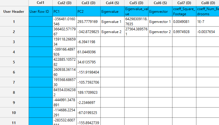
The output table contains the original input columns followed by the PCA-derived columns. For each row i and resolved component count k, the appended columns are:
| PC1…PCk | Projection scores — the coordinate of each sample along each principal component. |
| Eigenvalue | For rows 1 … k: the label “Eigenvalue 1” … “Eigenvalue k”. Empty for remaining rows. |
| Eigenvalue_value | For rows 1 … k: the numeric eigenvalue. Empty for remaining rows. |
| Eigenvector | For rows 1 … k: the label “Eigenvector 1” … “Eigenvector k”. Empty for remaining rows. |
| coeff_feature | For rows 1 … k: the loading coefficient of each input feature on that component. Empty for remaining rows. |
Example
Input
In the left-hand spreadsheet of the tab import the data.
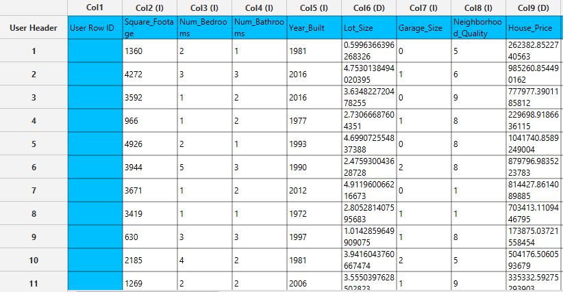
Configuration
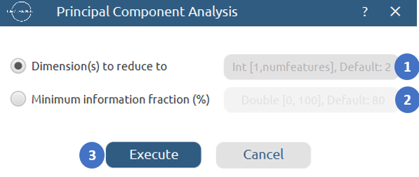
- Select
Data Transformation\(\rightarrow\)Dimensionality Reduction\(\rightarrow\)Principal Component Analysis - Choose the component selection mode:
- Select
Dimension(s) to reduce to[1] and enter a positive integer to fix the number of output components, or - Select
Minimum information fraction (%)[2] and enter a percentage; the algorithm will automatically determine how many components are needed.
- Select
- Click the
Executebutton [3] to run the algorithm.
Output
Once execution completes, the output will contain the original input columns alongside the PCA projection scores and, in the first k rows, the eigenvalues and eigenvector loadings for each retained component.
t-SNE
t-Distributed Stochastic Neighbour Embedding (t-SNE) is a non-linear dimensionality reduction technique that maps high-dimensional data to a low-dimensional embedding while preserving local neighbourhood structure. It converts pairwise similarities between points into conditional probabilities in the original space and minimises the divergence between those probabilities and their low-dimensional counterparts, producing a layout where nearby points in the original space remain nearby in the embedding. t-SNE belongs to the manifold learning family of methods and is particularly suited for visualisation of high-dimensional datasets.2
The algorithm models high-dimensional affinities with a Gaussian kernel and low-dimensional affinities with a Student-t kernel (heavy-tailed, degrees of freedom = 1). The heavier tail in the low-dimensional space alleviates the crowding problem by allowing moderately distant points to be placed further apart than a Gaussian would permit.
Pre-processing
Before computing affinities the input data is range-normalised: \(X \leftarrow \frac{X-\min(X)}{\max(X)-\min(X)}\) . This maps all values to [0, 1] and makes the perplexity parameter scale-independent.
High-dimensional affinities P
For each point i, a bandwidth parameter βi = 1 / (2σi²) is found by binary search so that the perplexity of the conditional distribution Pi matches the user-supplied perplexity value:
where d(·,·) is the chosen distance metric and H(Pi) is the Shannon entropy of Pi. The binary search runs for up to 50 iterations per point with a tolerance of 10−5.
The conditional probabilities are symmetrised and normalised to obtain the joint distribution: \(P_{ij}=\frac{p(j \mid i)+p(i \mid j)}{2n}\)
Low-dimensional affinities Q
In the embedding space, affinities are computed with a Student-t kernel: \(Q_{ij}= \frac{ \left(1+\lVert y_i-y_j\rVert^2\right)^{-1} }{ \sum_{a \ne b} \left(1+\lVert y_a-y_b\rVert^2\right)^{-1} }\)
Objective and gradient
The embedding is found by minimising the KL divergence between P and Q: \(C=\operatorname{KL}(P\parallel Q) = \sum_{i,j} P_{ij}\log\left(\frac{P_{ij}}{Q_{ij}}\right)\)
Optimisation
Gradient descent is run for the specified number of iterations using adaptive per-parameter gains and momentum:
\[v^{(t)} = \alpha v^{(t-1)} - \eta \, g \odot \nabla C\] \[y^{(t)} = y^{(t-1)} + v^{(t)}\]- Early exaggeration — P is multiplied by 4 for the first 100 iterations, then rescaled to 1, encouraging well-separated clusters to form early.
- Momentum schedule — momentum α starts at 0.5 and switches to 0.8 after iteration 20.
- Adaptive gains g — each gain is increased by 0.2 when the gradient and velocity have opposite signs, and multiplied by 0.8 otherwise, with a minimum of 0.01.
- Learning rate η is fixed at 500.
- The embedding is mean-centred after every iteration to prevent drift.
Use the t-SNE dimensionality reduction function by browsing in the top ribbon:
| Data Transformation \(\rightarrow\) Dimensionality Reduction \(\rightarrow\) t-SNE |
Input
The data input should consist of numerical instances, without any missing values. At least 2 numerical columns are required. There are no inherent limitations on the number of rows.
Configuration
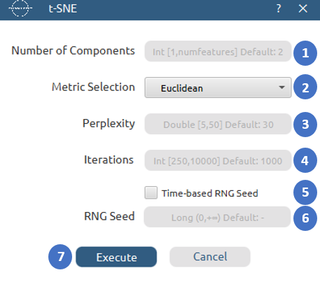
| Number of Components | Specify a positive integer in [1, number of features] representing the dimensionality of the target embedding. Default: 2. |
| Metric Selection | Choose the distance metric used when computing pairwise affinities in the original space. Available options: Euclidean, Manhattan. Default: Euclidean. |
| Perplexity | Specify a value in (0, 50] that controls the effective number of neighbours considered for each point. Default: 30. |
| Iterations | Specify a positive integer in [250, 10000] for the number of gradient descent steps. More iterations allow the embedding to converge more fully. Default: 1000. |
| Time-based RNG Seed | When checked, the random number generator is seeded with the current system time, producing a different initialisation on every run. When unchecked, the value in the RNG Seed field is used. |
| RNG Seed | Specify a non-negative integer seed to obtain a reproducible embedding. Active only when Time-based RNG Seed is unchecked. |
Output
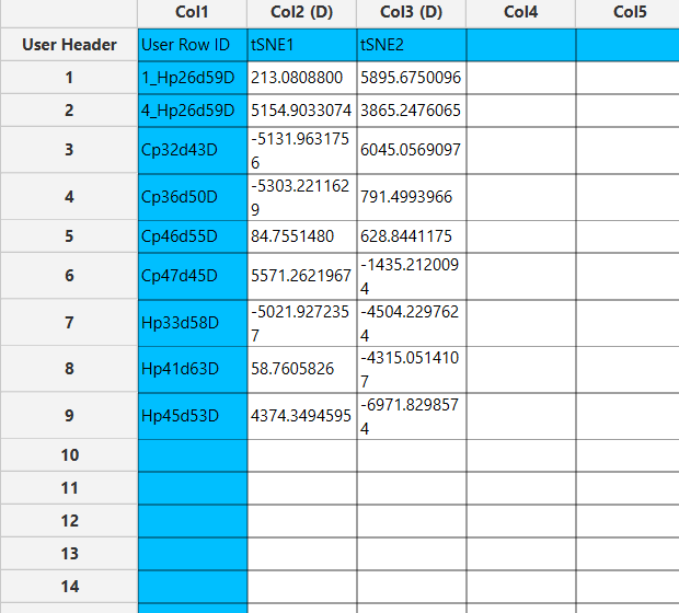
The output table contains the t-SNE embedding coordinates.
Example
Input
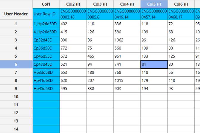
In the left-hand spreadsheet of the tab import the data.
Configuration
- Select
Data Transformation\(\rightarrow\)Dimensionality Reduction\(\rightarrow\)t-SNE - Set the
Number of Components[1] to define the dimensionality of the output embedding. - Choose a
Metric Selection[2] for computing pairwise distances in the original space. - Set the
Perplexity[3] to control the balance between local and global structure preservation. - Set the number of
Iterations[4] for the gradient descent optimisation. - Enable
Time-based RNG Seed[5] for a non-reproducible run, or leave it unchecked and specify a fixedRNG Seed[6] for reproducibility. - Click the
Executebutton [7] to run the algorithm.
Output
Once execution completes, the output will contain the t-SNE embedding coordinates (tSNE1, tSNE2, …).
UMAP
Uniform Manifold Approximation and Projection (UMAP) is a non-linear dimensionality reduction technique that maps high-dimensional data to a low-dimensional embedding while preserving both local neighbourhood structure and, to a greater extent than t-SNE, global topology. UMAP constructs a weighted graph (fuzzy simplicial set) that represents the manifold structure of the input data, then optimises a low-dimensional layout so that its own graph approximates the high-dimensional one as closely as possible. UMAP belongs to the manifold learning family of methods and is well suited for both visualisation and general-purpose dimensionality reduction. 3
Each point is connected to its nearest neighbours with edge weights that reflect local distance relative to the point’s own neighbourhood density. The resulting graph is then used to drive an embedding optimisation that balances attraction between connected points and repulsion between unconnected ones.
High-dimensional graph construction (fuzzy simplicial set)
For each point i the algorithm:
- Sorts all other points by distance and identifies ρi — the distance to the nearest non-zero neighbour (local connectivity offset).
- Finds a local scaling factor σi by binary search (64 iterations, tolerance 10−5) so that the sum of membership strengths over the k nearest neighbours equals log2(nNeighbors): \(v_{ij} = \begin{cases} 1, & d_{ij} \le \rho_i \\[4pt] \exp\left(-\dfrac{d_{ij}-\rho_i}{\sigma_i}\right), & d_{ij} > \rho_i \end{cases}\)
- Symmetrises the directed weights into an undirected fuzzy graph: \(W_{ij} = v_{ij} + v_{ji} - v_{ij}v_{ji}\)
Curve parameters a and b
A smooth curve \(f(x)=\frac{1}{1+a x^{2b}}\), is fitted to a piecewise target defined by the Min Distance and Spread parameters. The fitting uses a recursive grid search (up to depth 80, tolerance 10−8) that refines a 10×10 grid of (a, b) candidates by minimising the sum of squared residuals against 300 equally spaced evaluation points.
Embedding optimisation
The embedding is initialised by drawing each coordinate from a standard normal distribution using the specified seed. An edge schedule is built from the fuzzy graph: edges with weight below \(\frac{max(W)}{iterations}\) are discarded; surviving edges are assigned a sampling period proportional to \(\frac{\max(W)}{W_{ij}}\) .
Over the specified number of epochs, for each sampled positive edge (i, j) an attraction gradient is applied: \(\nabla_i^{+} = -\frac{ 2ab\,\lVert y_i-y_j\rVert^{2(b-1)} }{ 1+a\lVert y_i-y_j\rVert^{2b} } \,(y_i-y_j)\,\alpha\)
and for each negative sample k a repulsion gradient is applied: \(\nabla_i^{-} = \frac{ 2\gamma b }{ \left(0.001+\lVert y_i-y_k\rVert^2\right) \left(1+a\lVert y_i-y_k\rVert^{2b}\right) } \,(y_i-y_k)\,\alpha\)
All gradient values are clipped to [−4, 4] before the update. The learning rate decays linearly: \(\alpha_{\text{epoch}} = \alpha_0 \left( 1-\frac{\text{epoch}}{\text{iterations}} \right)\) Fixed optimisation constants: negative sample rate = 5, γ (repulsion strength) = 1.0, learning rate α0 = 1.0. The embedding is mean-centred once after all epochs.
Use the UMAP dimensionality reduction function by browsing in the top ribbon:
| Data Transformation \(\rightarrow\) Dimensionality Reduction \(\rightarrow\) UMAP |
Input
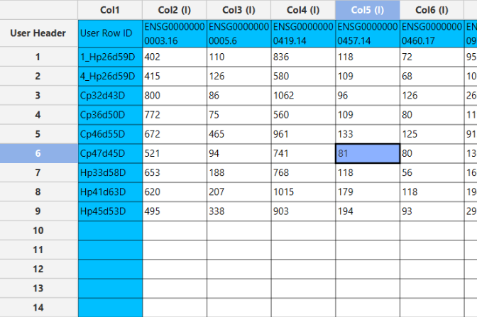
The data input should consist of numerical instances, without any missing values. At least 2 numerical columns are required. There are no inherent limitations on the number of rows.
Configuration
| Number of Components | Specify a positive integer in [1, number of features] representing the dimensionality of the target embedding. Default: 2. |
| Number of Neighbors | Specify a positive integer in [1, number of rows] controlling the size of the local neighbourhood used to build the fuzzy graph. Smaller values capture finer local structure; larger values capture broader global topology. Default: 15. |
| Metric Selection | Choose the distance metric used when computing pairwise distances in the original space. Available options: Euclidean, Manhattan. Default: Euclidean. |
| Min Distance | Specify a value in [0, 2] that controls how tightly points are packed in the embedding. Smaller values allow points to cluster more compactly; larger values push them apart, preserving more global structure. Default: 0.1. |
| Spread | Specify a value in [0, 5] that, together with Min Distance, determines the effective scale of the embedded clusters. The two parameters jointly define the shape of the low-dimensional membership curve. Default: 1.0. |
| Iterations | Specify a positive integer in [250, 10000] for the number of optimisation epochs. More epochs allow the embedding to converge more fully. Default: 1000. |
| Time-based RNG Seed | When checked, the random number generator is seeded with the current system time, producing a different initialisation on every run. When unchecked, the value in the RNG Seed field is used. |
| RNG Seed | Specify a non-negative integer seed to obtain a reproducible embedding. Active only when Time-based RNG Seed is unchecked. |
Output
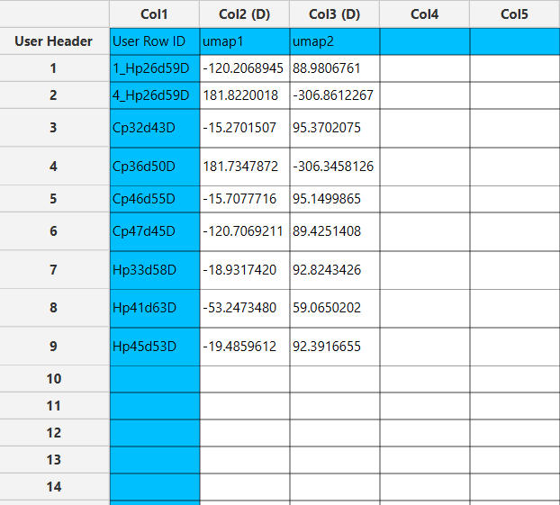
The output table contains the UMAP embedding coordinates.
Example
Input
In the left-hand spreadsheet of the tab import the data.
Configuration
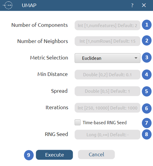
- Select
Data Transformation\(\rightarrow\)Dimensionality Reduction\(\rightarrow\)UMAP. - Set the
Number of Components[1] to define the dimensionality of the output embedding. - Set the
Number of Neighbors[2] to control the size of the local neighbourhood used during graph construction. - Choose a
Metric Selection[3] for computing pairwise distances in the original space. - Set
Min Distance[4] andSpread[5] to control the compactness and scale of the embedded clusters. - Set the number of
Iterations[6] for the optimisation. - Enable
Time-based RNG Seed[7] for a non-reproducible run, or leave it unchecked and specify a fixedRNG Seed[8] for reproducibility. - Click the
Executebutton [9] to run the algorithm.
Output
Once execution completes, the output will contain the UMAP embedding coordinates (UMAP1, UMAP2, …).
Tips
PCA:
- Consider data scaling prior to applying PCA, as the algorithm is sensitive to the scale of input features. Variables with larger numeric ranges will otherwise dominate the principal components regardless of their informational content.
- Use the Minimum information fraction mode when you do not have a specific target dimensionality in mind. A threshold of 80–95% is a common starting point that balances information retention with dimensionality reduction.
- PCA produces a linear projection. If the data lies on a non-linear manifold, consider t-SNE or UMAP instead.
t-SNE:
- t-SNE is primarily a visualisation tool. For downstream tasks such as clustering or classification, consider using the original features or a linear reduction such as PCA as input.
- Perplexity is the most influential parameter. Values in the range 5–15 emphasise fine local cluster structure; values in the range 30–50 produce smoother, more globally coherent layouts. It is advisable to try several values and compare the resulting embeddings.
UMAP:
- Consider data scaling prior to applying UMAP, as pairwise distances are computed directly from the raw feature values. Features with larger numeric ranges will otherwise dominate the neighbourhood graph construction.
- Number of Neighbors is the most influential parameter. Small values (5–10) capture fine local structure and produce tightly separated clusters; large values (30–100) incorporate more global topology and yield smoother, more connected layouts.
- Min Distance controls cluster compactness in the embedding. Small values (e.g. 0.0–0.1) pack points tightly together, making cluster boundaries sharper; larger values (e.g. 0.5–1.0) spread points out, which can help reveal continuous structure within clusters.
- For large datasets, UMAP is generally faster than t-SNE for equivalent embedding quality, making it more practical when iteration over parameters is needed.
See also
The model generated by a dimensionality reduction function can be applied to any compatible input dataset through Existing Model Utilization. For example, a dimensionality reduction model fitted to the training set can be used to project test or external datasets into the same reduced-dimensional feature space.
References
- Wold, Svante, Kim Esbensen, and Paul Geladi. Principal component analysis. Chemometrics and Intelligent Laboratory Systems; 1987; 2(1–3): 37–52. https://doi.org/10.1016/0169-7439(87)80084-9. van der Maaten, Laurens, and Geoffrey
- van der Maaten, Laurens, and Geoffrey Hinton. Visualizing data using t-SNE. Journal of Machine Learning Research; 2008; 9: 2579–2605. https://www.jmlr.org/papers/volume9/vandermaaten08a/vandermaaten08a.pdf.
- McInnes, Leland, John Healy, and James Melville. UMAP: Uniform Manifold Approximation and Projection for Dimension Reduction. arXiv; 2020; arXiv:1802.03426. https://arxiv.org/pdf/1802.03426.
Version History
Introduced in Isalos Analytics Platform v2.1.2
Instructions last updated on August 2026