









SHAP Analysis
SHAP analysis is a model explanation tool used to break down a model prediction into feature-level contributions. Instead of only reporting the final prediction, SHAP assigns each input feature a value describing how much that feature moved the prediction away from a reference value. This helps identify which variables support, oppose, or have little effect on a prediction for each row of data.
In Isalos, SHAP analysis is available for several model families through both model-agnostic and model-specific explanation methods. Model-agnostic methods, such as Kernel SHAP and Permutation SHAP, explain a fitted model by repeatedly evaluating it under different feature-substitution scenarios. Model-specific methods, such as Linear SHAP, Tree SHAP, and Deep SHAP, use the structure of the fitted model directly to calculate explanations more efficiently or more exactly for supported models.
Use SHAP Analysis by browsing in the top ribbon:
| Statistics \(\rightarrow\) SHAP Analysis |
Mathematical Background
SHAP is based on Shapley values from cooperative game theory.1 In the SHAP setting, the “game” is the model prediction and the “players” are the input features. The objective is to distribute the difference between a reference prediction and the prediction for the row being explained among the model input features.2
SHAP explains one scalar model output at a time. For regression models this scalar is usually the predicted response. For classification models it is usually the probability or score of one explained class. If a model produces several outputs, the SHAP values shown in one output table refer only to the scalar output selected internally by the SHAP method and model adapter.
For a model prediction \(f(x)\), SHAP explanations are commonly written as:
where \(M\) is the number of model input features, \(\phi_0\) is the reference or baseline value, and \(\phi_j\) is the contribution assigned to feature \(j\).
The baseline \(\phi_0\) is the prediction expected before seeing the explained row. The SHAP values then describe how the features of the explained row move the model away from this baseline. A positive SHAP value increases the explained scalar prediction relative to the baseline, while a negative SHAP value decreases it.
The classical Shapley value for feature \(j\) is:
where \(F\) is the full set of model features, \(S\) is a subset of features that does not include feature \(j\), \(v(S)\) is the model output assigned to the feature coalition \(S\), and \(v(S \cup \{j\}) - v(S)\) is the marginal contribution of adding feature \(j\) to coalition \(S\).
The practical challenge in predictive modeling is that most models cannot directly evaluate a row with a feature “missing”. SHAP methods therefore differ mainly in how they define and compute the value function \(v(S)\). This is the missing-feature problem.
The most important property for interpretation is the efficiency property:
Isalos checks this reconstruction numerically and reports the result once in the output table’s reporting box, together with the maximum absolute residual and the tolerance. The check applies to the scalar named in Output Space; for example, class-probability contributions reconstruct a probability, while raw-margin contributions reconstruct a margin. Passing this check confirms numerical reconstruction, but does not by itself establish that sampled attributions have converged or that the chosen background population is appropriate. See How to Read SHAP Tables.
The Missing-Feature Problem
When a feature is absent from a coalition, the model still requires a complete input vector. SHAP methods solve this by defining how missing features are represented during explanation. This is why Isalos exposes different configuration options for different SHAP methods.
In model-agnostic methods, missing features are usually replaced using values from a background dataset. The background dataset represents the reference population against which explanations are computed. For example, if feature \(x_j\) is considered absent, Kernel SHAP or Permutation SHAP can replace it with values sampled from the background rows while keeping the present features fixed.
In model-specific methods, the fitted model structure is used directly. Linear SHAP uses fitted coefficients and a reference feature distribution. Tree SHAP uses tree paths and node statistics. Deep SHAP uses layer-by-layer contribution propagation through a fitted neural network. These approaches still require a clear baseline, but they avoid brute-force feature coalition evaluation where the model structure permits a more direct calculation.
For a background dataset \(B = \{b^{(1)}, b^{(2)}, \ldots, b^{(N_B)}\}\), a common model-agnostic value function for row \(x\) and coalition \(S\) is:
where the hybrid row \(h_S(x,b)\) is:
This means that present features come from the row being explained, while absent features come from one background row. Averaging over background rows approximates the expected prediction for the coalition. Kernel SHAP and Permutation SHAP use this idea directly. Linear SHAP, Tree SHAP, and Deep SHAP specialize the baseline and contribution calculation to the fitted model family.
Choosing the Background Dataset
The background dataset should be interpreted as the reference population for the explanation. It is not simply an additional input table. It defines the baseline prediction and, for methods that substitute missing features, it also defines the values used when a feature is treated as absent.
Isalos allows the background dataset to be selected independently from the dataset used to train the model. This is intentional. It gives the user control over the reference population, allows smaller representative background subsets to be used for efficient computation, and supports imported or pre-trained models whose original Isalos training datasheet may not be available.
Choose representative rows from the population against which predictions should be interpreted, using the model’s feature names, units, encodings and preprocessing. Training, validation/test or deployment data can supply this reference population; a held-out dataset is not automatically a better SHAP background because it was excluded from model fitting. Keep the role of the background separate from the role of a held-out test set used to assess predictive performance.
Using complete background rows retains the relationships among the features replaced together. However, combining those values with the query’s retained features can break relationships between the two groups and create combinations that are uncommon in the original data. Background substitution does not generally compute a conditional distribution of missing features given the present features. This distinction matters for strongly dependent inputs, and a larger background does not remove it.
For imported Isalos-compatible fitted models, supply a compatible background datasheet when the selected SHAP method requires one. The original training datasheet need not be present in the project. Tree SHAP models with sufficient stored path statistics can be explained without a separately supplied background. Importing a model does not mean that arbitrary external formats, such as a Keras model file, are accepted by Isalos.
SHAP Methods Available in Isalos
The SHAP type shown in the configuration window depends on the selected model. Isalos prioritizes the model-specific method when one is available, while still allowing Kernel SHAP or Permutation SHAP for many supported model families.
| SHAP method | Main idea | Background/reference data | Sampling budget field | Typical supported model family |
|---|---|---|---|---|
| Kernel SHAP | Model-agnostic Shapley approximation using weighted coalitions | Required | Number of Coalition Samples | Supported fallback for XGBoost, Random Forest, J48, Linear SGD, kNN, MLP, RBF, MLR, GLM, GEE, and Random Tree models |
| Permutation SHAP | Model-agnostic attribution by feature reveal orderings | Required | Number of Permutations | Supported fallback for the same model families; default SHAP option for RBF models |
| Linear SHAP | Uses fitted linear coefficients and reference values | Required | Not shown | MLR and Linear SGD regression models |
| Tree SHAP | Uses tree structure and path statistics | Usually not required; Random Forest may require reference rows | Not shown | Random Forest, J48, Random Tree, and compatible XGBoost classification/regression tree models |
| Deep SHAP | Uses fitted MLP layers and background-based baselines | Required | Not shown | Multi-Layer Perceptron models |
Both k-Nearest Neighbors (kNN) and k-Nearest Neighbors (kNN) NEW support Kernel SHAP and Permutation SHAP, with Kernel SHAP selected by default. Select the exact fitted model intended for the explanation: the two kNN implementations can produce different predictions and consequently different SHAP values. Their shared eligibility does not imply numerical equivalence.
The sampling-budget field is visible only for Kernel SHAP and Permutation SHAP. Deep SHAP, Linear SHAP, and Tree SHAP do not use a coalition or permutation budget in the SHAP configuration window.
After a model is selected, Isalos automatically selects the best-fitting compatible SHAP type for that model family. This automatic selection is intended to guide the user toward the most appropriate available method without requiring them to know the implementation details. For example, a supported MLP model is directed toward Deep SHAP, a supported linear model is directed toward Linear SHAP, and supported tree models are directed toward Tree SHAP when the model-specific compatibility checks are satisfied.
Query and background tables must contain the fitted model’s input features with compatible datatypes. Numeric feature columns may be Integer or Double; an Integer model feature must be supplied without fractional values. Additional target or identifier columns are not explanation features unless they were actually used to train the model.
The selected SHAP type can still be reviewed and changed when alternative compatible methods are available. The model-agnostic methods remain useful when the user wants a method with a different missing-feature interpretation or when a model-specific compatibility check is not satisfied. In the method-specific examples below, “select” the SHAP type should therefore be read as “confirm the auto-selected option or choose this method deliberately if another compatible option is currently selected.”
Selecting Features for the Beeswarm Plot
After ticking Beeswarm Plot, the Select Features button appears below it. Choose the features to display, or leave the selection unspecified to show the ten features with the largest mean absolute SHAP values across the query rows. If fewer than ten features are available, all are shown.
This selection controls the plot only. SHAP still explains all model input features and exports all feature contributions in the table. The selector inside the Beeswarm window allows features to be added or removed afterward. See Beeswarm Plot for interpretation and display controls.
Example Datasets and Configuration Hints
The method examples use small synthetic datasets for illustrating the workflow, not for assessing model accuracy. Each training dataset has 100 rows and each test dataset has 12 rows. The five input features are Temperature, Pressure, Concentration, Duration, and Flow. They are min-max scaled using the training-set bounds; the test data uses the same transformation. The final column is the unscaled target: Response for regression or Class (0/1) for classification. Do not include the target or the worksheet’s User Row ID column among model input features.
The screenshots show some fields before values have been entered. Light-grey text is a placeholder, not a configured value. A numerical Default in a sampling-budget field is used when that field is left blank. In contrast, Background Size (Rows) shows Default: -: enter a valid number before executing. For these examples, enter 100 to use all rows of train_reg or train_class. The displayed interval [1, 100] describes the valid range; it does not select 100 automatically.
Kernel SHAP
Kernel SHAP is a model-agnostic SHAP method. It treats the selected model as a prediction function and estimates feature contributions by evaluating masked versions of the input row. Each masked row represents a coalition of present features, while missing features are supplied from the selected background dataset.2
Kernel SHAP is useful when no exact model-specific SHAP implementation is available. The advantage is generality: the method only needs to call the fitted model. The cost is computational: the method must evaluate many hybrid rows and then solve a weighted regression problem for each explained row.
Mathematical Formulation
Kernel SHAP fits a local additive explanation model around the row being explained. A coalition is represented by a binary vector \(z \in \{0,1\}^{M}\), where \(z_j = 1\) means feature \(j\) is present and \(z_j = 0\) means feature \(j\) is absent.
The local explanation model is:
For each coalition \(z\), the model-agnostic coalition value is computed by replacing absent features with background values:
The SHAP values are obtained by fitting \(g(z)\) to the coalition values using the Shapley kernel. In Kernel SHAP, the Shapley kernel is the coalition-weighting function \(\pi(z)\). For a coalition with size \(s = \sum_j z_j\), where \(0 < s < M\):
The weighted least-squares objective is:
subject to the SHAP efficiency constraint:
In Isalos, the baseline is:
Background Interpretation
The background dataset defines what “missing” means. If a feature is excluded from a coalition, Isalos substitutes the feature value from each selected background row and averages the resulting predictions. The explanation is therefore relative to the selected background population, not relative to an abstract zero vector.
This is important in practice:
- A background set drawn from the model’s training distribution usually gives explanations relative to typical modeled data.
- A very small or unrepresentative background set can shift the baseline and change the apparent contributions.
- Background rows must contain the same model input feature names as the selected model. Extra columns are ignored.
Computational Technique in Isalos
For each query row, Isalos executes Kernel SHAP as follows:
- Compute the baseline prediction as the mean prediction over the selected background rows.
- Compute the full prediction \(f(x)\) for the query row.
- Build a coalition set according to the requested coalition-sample budget.
- Give high-weight coalition sizes priority. Small coalitions and their large-complement counterparts are enumerated first when the budget permits.
- Use random sampling for the remaining middle coalition sizes when the requested budget is smaller than the full coalition space.
- For every coalition, build a batch of hybrid rows by combining the query row with each selected background row.
- Average the model predictions for those hybrid rows to obtain the coalition value \(v_x(z)\).
- Solve the weighted least-squares system with the efficiency constraint applied algebraically.
Each evaluated non-trivial coalition becomes one row in a local regression problem. The row records which features were present in that coalition. The target is not the raw coalition prediction itself, but the coalition prediction measured relative to the baseline:
This centering step is important because SHAP explains a prediction difference, not an absolute prediction. The baseline \(\phi_0\) represents the model output before the explained row’s feature values are introduced. When all features are present, the coalition value is the full prediction \(f(x)\), so the feature contributions must reconstruct the movement from the baseline to the full prediction. The full prediction difference for the query row is:
The efficiency constraint requires the feature contributions to sum to this full prediction difference:
For one coalition mask \(z\), Kernel SHAP then uses a local additive surrogate:
In this equation, \(z_j\) is only a coalition indicator. If \(z_j=1\), feature \(j\) is present in the surrogate model and its contribution \(\phi_j\) is included in the sum. If \(z_j=0\), feature \(j\) is absent from the coalition and its contribution is excluded from that surrogate row. The approximate equality has two practical meanings. First, \(v_x(z)\) is usually estimated from a finite number of background rows rather than the full population distribution. Second, for nonlinear models or models with feature interactions, one fixed additive vector \(\phi\) cannot usually reproduce every coalition value exactly. Kernel SHAP therefore fits the best local additive explanation under the Shapley-kernel weighting scheme.
After the non-trivial coalitions are generated, Isalos stacks the coalition rows into a matrix problem. Let \(Z\) be the coalition-design matrix, where row \(i\) contains the mask values for coalition \(z^{(i)}\). Let \(y\) be the vector of centered coalition targets, where \(y_i = y(z^{(i)})\). If \(\phi\) is the vector of feature contributions, the residual for row \(i\) is:
The Shapley kernel assigns a weight \(w_i = \pi(z^{(i)})\) to each coalition row. These weights are collected in a diagonal matrix \(W\). A weighted least-squares solve minimizes:
This weighted problem can be written as an ordinary least-squares problem after rescaling each row. If row \(i\) of the design matrix and target vector are multiplied by \(\sqrt{w_i}\), the residual for that row becomes \(\sqrt{w_i}r_i\). Squaring it gives:
This is why the matrix form uses \(\sqrt{W}\) rather than \(W\) directly. Multiplying by \(\sqrt{W}\) rescales each coalition row by the square root of its Shapley-kernel weight before the least-squares solve. High-weight coalitions therefore have a stronger influence on the fitted local explanation, while low-weight coalitions have less influence.
Kernel SHAP also needs the final explanation to satisfy the efficiency constraint exactly. This anchors the local explanation to two fixed endpoints: the empty coalition corresponds to the baseline difference \(0\), and the grand coalition corresponds to the full prediction difference \(d=f(x)-\phi_0\). Rather than solving all \(M\) feature contributions independently and then correcting the sum afterward, Isalos removes one contribution from the set of free unknowns. This constrains the solver so the fitted explanation cannot drift away from the required full-coalition reconstruction. For one eliminated feature \(k\):
Substituting this expression into each coalition row changes the local model into a reduced row equation. For coalition row \(i\), with mask \(z^{(i)}\) and centered target \(y_i = y(z^{(i)})\):
Here, \(z^{(i)}_k\) and \(d\) are scalars, so \(z^{(i)}_k d\) is also scalar. The vector notation only appears after these row equations are stacked. The reduced system solves only for the \(M-1\) free contributions. Let \(\phi_{\setminus k}\) be the vector containing all feature contributions except the eliminated contribution \(\phi_k\). Let \(Z_{\mathrm{red}}\) be the reduced coalition-design matrix whose row entries are \(z^{(i)}_j-z^{(i)}_k\) for \(j \neq k\). Let \(y_{\mathrm{red}}\) be the adjusted target vector whose row entries are \(y_i-z^{(i)}_kd\). This makes the reconstruction property part of the solve itself: once \(\phi_{\setminus k}\) is found, the omitted contribution \(\phi_k\) is recovered from the efficiency equation.
Putting these pieces together, the reduced weighted least-squares problem solved by Isalos is:
Isalos solves this reduced weighted system using singular-value decomposition, which improves numerical stability when coalition rows are nearly collinear or the design matrix is close to rank deficient.
Kernel SHAP does not evaluate the empty coalition or the grand coalition as ordinary sampled coalition rows. The empty coalition is represented by the baseline \(\phi_0\), and the grand coalition is represented by the full prediction \(f(x)\) and the efficiency constraint. Therefore the number of non-trivial coalition masks available for the weighted regression is:
If \(C_{\mathrm{budget}}\) is the requested number of coalition samples, the number of evaluated non-trivial coalition masks is bounded by:
In exact-enumeration cases, \(C_{\mathrm{eff}} = 2^M - 2\). In sampled cases, the requested budget acts as the maximum number of non-trivial coalition masks used by the regression.
For \(N_{\mathrm{query}}\) explained rows and \(N_B\) background rows, the dominant model-evaluation workload scales approximately as:
This is why the coalition budget and background size are visible configuration choices for Kernel SHAP.
Using Kernel SHAP in Isalos
Input
Kernel SHAP requires a query datasheet and a background datasheet. The query datasheet contains the rows to be explained and must include the selected model’s input feature columns. The background datasheet is selected independently and should represent the reference population for the explanation. It must contain the same model input features because it supplies replacement values for missing coalition features. Choose a representative reference population as described in Choosing the Background Dataset. For imported or pre-trained models, upload an appropriate background datasheet with the same feature preprocessing expected by the model. Extra columns may be present in either sheet, but they are ignored during the SHAP calculation.
Configuration
| Configuration field | Description |
|---|---|
| Select Model | Select the fitted model to explain. |
| Select SHAP Type | Confirm or choose Kernel SHAP. Isalos may auto-select another compatible method first when it is a better fit for the selected model. |
| Select Background | Select the reference dataset used to replace missing features during coalition evaluation. Follow Choosing the Background Dataset, including for imported models. |
| Background Size (Rows) | Select the number of rows to use from the background dataset. |
| Number of Coalition Samples | Select the coalition sampling budget. Larger values can improve stability but increase runtime. |
| Beeswarm Plot | Generate a plot using the display selection described in Beeswarm Plot. |
| Select Features | Shown when Beeswarm Plot is ticked. Choose displayed features, or retain the default top ten. This does not limit the SHAP calculation. |
Output
The Kernel SHAP output table contains the explained prediction, the baseline value, the efficiency check, and one SHAP-value column for each model input feature. The explanation is relative to the selected background rows and the requested coalition-sample budget.
Example
This example explains a fitted kNN regression model trained on the 100-row regression datasheet. The same datasheet, named train_reg, supplies the background/reference rows. The separate 12-row test datasheet contains the queries to be explained. Model training is completed before opening SHAP Analysis.
Input
Prepare the 100-row regression training datasheet and the 12-row test datasheet, with the five input features and the Response target described above. Here, the training datasheet also represents the reference population for Kernel SHAP.
The background/training datasheet and the test/query datasheet must contain the same model input feature columns. The response column may be present, but SHAP uses the fitted model inputs when constructing explanations.
The first rows of the 100-row regression training/background datasheet are shown below.

The 12-row test datasheet containing the rows to be explained is shown below.

Configuration
Use Kernel SHAP by selecting:
| Statistics \(\rightarrow\) SHAP Analysis \(\rightarrow\) Select SHAP Type: Kernel SHAP |
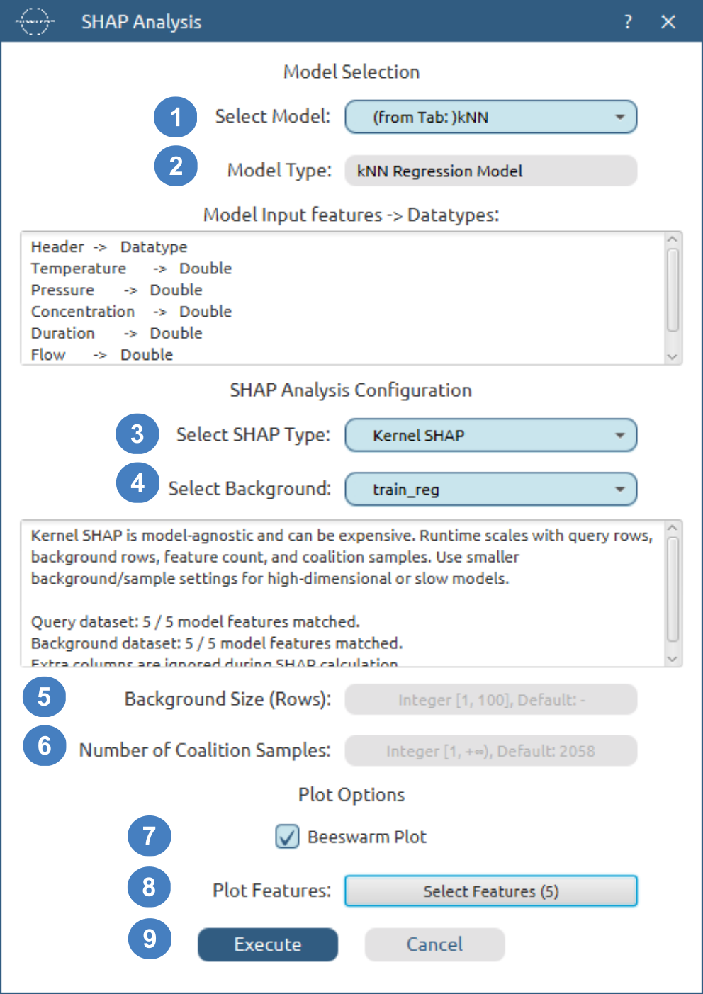
Select Modelis used to choose the already fitted kNN regression model that will be explained.Model Typeconfirms that the selected model is a kNN model. This helps verify that the SHAP configuration is being applied to the intended fitted model.Select SHAP Typeis set toKernel SHAP. If Isalos auto-selects another compatible SHAP type after model selection, confirm or change the selection here.Select Backgroundis set totrain_reg. This supplies the reference rows used when Kernel SHAP substitutes values for missing coalition features.Background Size (Rows)is blank in the screenshot. Enter100to use the full training background, or a smaller positive count to sample fewer reference rows.Default: -indicates that no automatic count is supplied.Number of Coalition Samplesis left blank to use the displayed default of2058. For five input features, this follows the practical rule \(2M+2^{11}=2058\), also documented for Python SHAP’s KernelExplainer.3 This is a budget, not a promise to evaluate 2058 distinct masks: with five varying features, only \(2^5-2=30\) non-trivial coalitions exist. Fewer varying features reduce this further. The empty and full coalitions supply the constraints described in the computational method.Beeswarm Plotis enabled so that Isalos also produces a global summary plot after the SHAP table is generated. The plot interpretation is shared across SHAP methods and is described later in the Beeswarm Plot section.Plot Features: Select Features (5)opens the feature selector. Five features are selected for display in this screenshot. This selection does not restrict the features explained in the output table.Executestarts the Kernel SHAP calculation.
The Model Input Features -> Datatypes panel lists the five fitted inputs as Double. The message panel below the background selector summarizes the runtime warning and confirms that the query and background datasets each match all five model features. Extra columns, such as the target, are ignored by the SHAP calculation.
Output
The output is a regression SHAP table. Each row corresponds to one explained test row. The prediction column contains the kNN regression prediction for that test row, base_value is the mean prediction over the selected background rows, and the feature-level SHAP columns show how each input feature moves the prediction away from that background baseline.
Inspect the SHAP output table by checking that the displayed prediction is reconstructed by the baseline plus the feature-level SHAP values. Positive feature SHAP values increase the explained regression prediction relative to the baseline, while negative values decrease it.
The reporting box’s Efficiency Check summarizes reconstruction across all 12 queries. The columns φ_Temperature, φ_Pressure, φ_Concentration, φ_Duration, and φ_Flow report contributions for the five inputs, in regression-response units. See How to Read SHAP Tables for the shared layout.
The completed example is shown below. Click the image to inspect the full-size table.
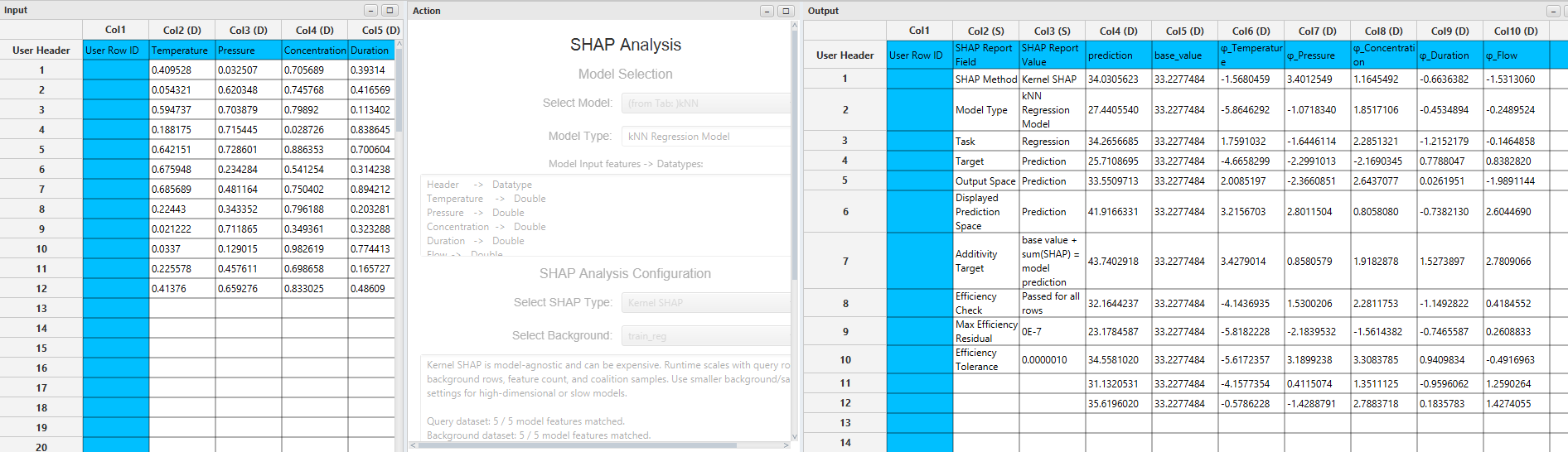
The common base_value is approximately 33.2277484. For the first query, the five contributions sum to approximately 0.8028139, giving the displayed prediction 34.0305623 when added to the baseline. The reporting box states Passed for all rows under Efficiency Check, with a tolerance of 0.0000010. Its residual is displayed as 0E-7; this is a formatted numerical result, not a claim of exact arithmetic. The predicted response need not equal the observed Response target: SHAP reconstructs the fitted model’s prediction, not the ground-truth value.
If Beeswarm Plot was selected, see Beeswarm Plot for a shared example, interpretation and display controls.
Permutation SHAP
Permutation SHAP is a model-agnostic method that estimates feature contributions by repeatedly revealing features in different orders. For each sampled ordering, the method starts from background rows, inserts the explained row’s feature values one by one, and records the marginal prediction change assigned to the feature that was just revealed. Averaging these marginal changes across orderings and background rows estimates the contribution of each feature.4
Like Kernel SHAP, Permutation SHAP uses a background dataset to represent missing features. The conceptual difference is in how the Shapley averaging is approximated. Kernel SHAP fits a weighted coalition regression, while Permutation SHAP estimates Shapley values directly from sampled feature orderings. In Isalos, this makes Permutation SHAP the default choice for Radial Basis Function (RBF) models. RBF models are nonlinear, distance-based predictors whose behavior depends on centers, widths, and radial kernel responses. They do not fit the assumptions of the implemented Linear SHAP, Tree SHAP, or Deep SHAP paths. Permutation SHAP can still explain them because it only needs reliable model predictions for complete rows and a representative background dataset for missing-feature substitution. Kernel SHAP remains available as an alternative model-agnostic method, but Permutation SHAP is the default RBF choice because it avoids an additional weighted surrogate-regression solve and keeps the explanation tied to direct reveal-order prediction differences.
Mathematical Formulation
Let \(A(x,B)\) be the active feature set for query row \(x\) and selected background dataset \(B\). A feature is active when at least one selected background row differs from the query row for that feature beyond a small numerical tolerance. Features that do not vary between the query row and all selected background rows cannot change any masked row, so they receive zero contribution in the permutation calculation.
Let \(\pi\) be a sampled ordering of the active features. For feature \(j\), define \(P_j^\pi\) as the set of active features that appear before \(j\) in the ordering \(\pi\). The permutation-based Shapley contribution can be written as:
Using background rows, the coalition value for a set of revealed features \(S\) is:
Here, \(h_S(x,b^{(i)})\) is the hybrid row whose features in \(S\) come from the query row \(x\) and whose remaining features come from background row \(b^{(i)}\). Thus, missing features are not set to zero; they are supplied by reference rows.
For one background row \(b\) and one feature order \(\pi\), define:
The forward marginal contribution for the feature at position \(k\) is:
The forward pass telescopes from the background row to the query row:
Isalos also evaluates the reverse removal direction along the same path. The reverse pass starts from the full query row and removes active query features back to the background row. For feature \(\pi_k\), the reverse contribution is the same path difference written from the removal direction:
The forward and reverse passes make the full path reconstruction explicit for every background row. After averaging, the feature contributions reconstruct the difference between the query prediction and the background baseline:
The approximation reflects the fact that only sampled feature orderings and selected background rows are used.
Background Interpretation
The background dataset defines the starting point for each reveal ordering. For each selected background row, Isalos begins from the background row, inserts query feature values according to a sampled ordering, and measures how the prediction changes as the row becomes more like the query row.
The resulting explanation answers the question:
On average, how much does each feature contribute when the query row is built from representative background rows?
For RBF models, this background interpretation is especially important. RBF predictions depend on distances between the query row and fitted radial centers. Replacing absent query features with background values creates hybrid rows that remain in the same feature space and preserve realistic feature scales. If the background dataset is poorly chosen, the hybrid rows may no longer represent meaningful locations for the RBF predictor. Use a representative, compatibly preprocessed reference dataset; see Choosing the Background Dataset.
Permutation SHAP is stochastic. Increasing the number of permutations generally improves stability, but the improvement is gradual and runtime increases directly with the requested permutation count.
Computational Technique in Isalos
For each query row, Isalos executes Permutation SHAP as follows:
- Compute the baseline prediction as the mean prediction over the selected background rows.
- Identify active features. A feature is active when its query value differs from at least one selected background value beyond a small numerical tolerance.
- Sample feature orderings only over the active features.
- For each sampled ordering and each background row, evaluate a forward reveal pass from background to query.
- Evaluate a reverse removal pass from query back to background using the same ordering.
- Add the forward and reverse marginal changes for each feature.
- Average across both directions, all sampled permutations, and all background rows.
If \(A\) is the number of active features and \(P\) is the effective number of sampled permutations, each background row contributes approximately:
model states per permutation. Across \(N_B\) background rows, the model-evaluation workload scales approximately as:
Inactive features receive zero contribution because they do not change the masked rows generated from the selected background data. This is both a numerical optimization and an interpretability safeguard: a feature that is identical between the query row and all selected background rows has no reveal event to attribute in the selected reference context.
For one query row, the final contribution for feature \(j\) can be viewed as the average of all observed forward and reverse marginal changes:
This explicit averaging step is the reason the number of permutations controls both runtime and Monte Carlo stability. Because the estimator samples reveal orderings, two runs with very small permutation counts can differ slightly even when the same model and datasets are used. Increasing the permutation count gives a denser sample of possible feature orderings.
Using Permutation SHAP in Isalos
Input
Permutation SHAP requires a query datasheet and a background datasheet. The query datasheet contains the rows to be explained, while the independently selected background datasheet defines the reference rows from which query features are revealed. Both datasets must contain the selected model’s input feature columns. Choose the reference population deliberately; see Choosing the Background Dataset. For imported or pre-trained models, upload a compatible background dataset with the same preprocessing expected by the model. Extra columns are ignored.
Configuration
| Configuration field | Description |
|---|---|
| Select Model | Select the fitted model to explain. For the example below, this is an RBF regression model. |
| Select SHAP Type | Confirm or choose Permutation SHAP. For RBF models, Isalos auto-selects Permutation SHAP by default and also keeps Kernel SHAP available as an alternative. |
| Select Background | Select the reference dataset used to replace missing features during permutation evaluation. Follow Choosing the Background Dataset, including for imported models. |
| Background Size (Rows) | Select the number of rows to use from the background dataset. |
| Number of Permutations | Select the number of feature orderings to evaluate. Larger values improve stability but increase runtime. |
| Beeswarm Plot | Generate a plot using the display selection described in Beeswarm Plot. |
| Select Features | Shown when Beeswarm Plot is ticked. Choose displayed features, or retain the default top ten. This does not limit the SHAP calculation. |
Output
The output table contains the explained prediction or class probability, baseline, efficiency check, and one SHAP-value column per model input feature. The explanation is stochastic because it averages over sampled feature orderings; larger permutation counts usually improve stability. For classification models, the SHAP values explain the displayed scalar class probability, not the entire multi-class probability vector at once.
Example
Input
This example explains an RBF regression model trained on the 100-row regression datasheet. Select that datasheet, train_reg, as the background/reference source and use the separate 12-row regression test datasheet as the query input.
The first rows of the regression training datasheet used as the background/reference data are shown below.
The regression test datasheet contains the 12 query rows to be explained.
Configuration
Use Permutation SHAP by selecting:
| Statistics \(\rightarrow\) SHAP Analysis \(\rightarrow\) Select SHAP Type: Permutation SHAP |
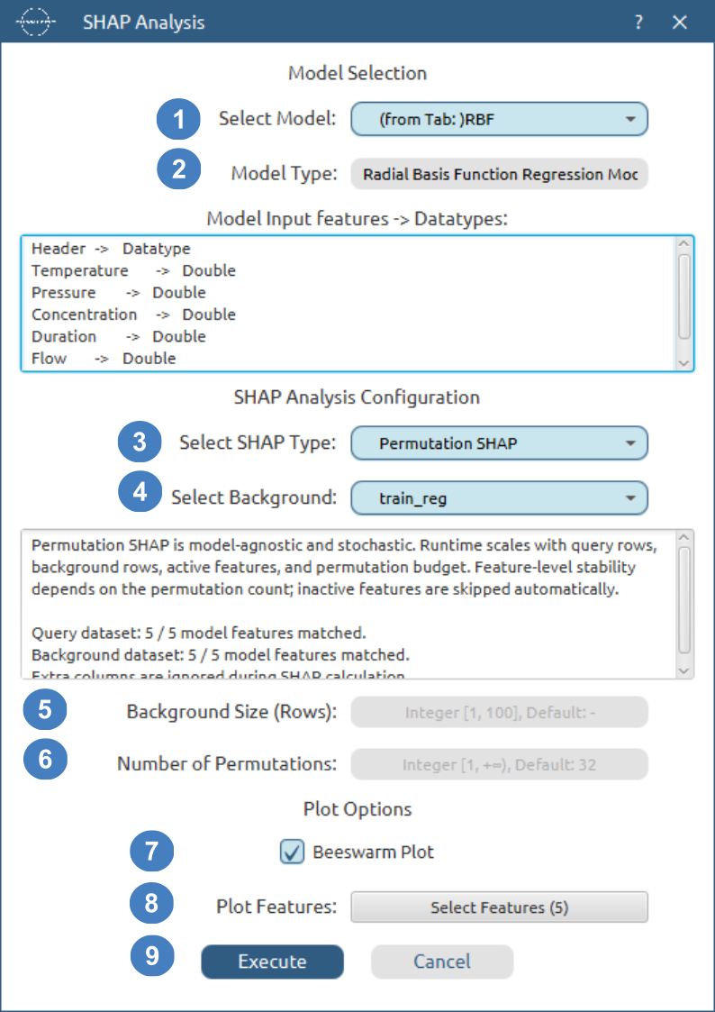
Select Modelchooses the fitted model in theRBFtab.Model Typeidentifies it as a Radial Basis Function regression model.- Confirm or choose
Permutation SHAP. For RBF models, this is the default SHAP type selected by Isalos. Select Backgroundis set totrain_reg.Background Size (Rows)shows the valid range[1, 100]andDefault: -. Enter100before execution to use all reference rows; the screenshot shows the placeholder, not an entered count.Number of PermutationsshowsDefault: 32. Leave the field blank to use 32 sampled orderings or enter another positive count. This controls permutation sampling, not the number of features.- Optionally select
Beeswarm Plot. If enabled, interpret the generated plot using the shared Beeswarm Plot section. Plot Features: Select Features (5)opens the selector; all five inputs are selected for this display. The output table still explains every input feature.- Click
Execute.
Output
The output is a regression SHAP table with one explanation for each of the 12 test rows. prediction contains the fitted RBF response, base_value is the mean response over the selected background rows, and the five feature-level columns explain the difference from that baseline. For an RBF classification model instead, the explained scalar would be a class probability, as indicated in the reporting box.
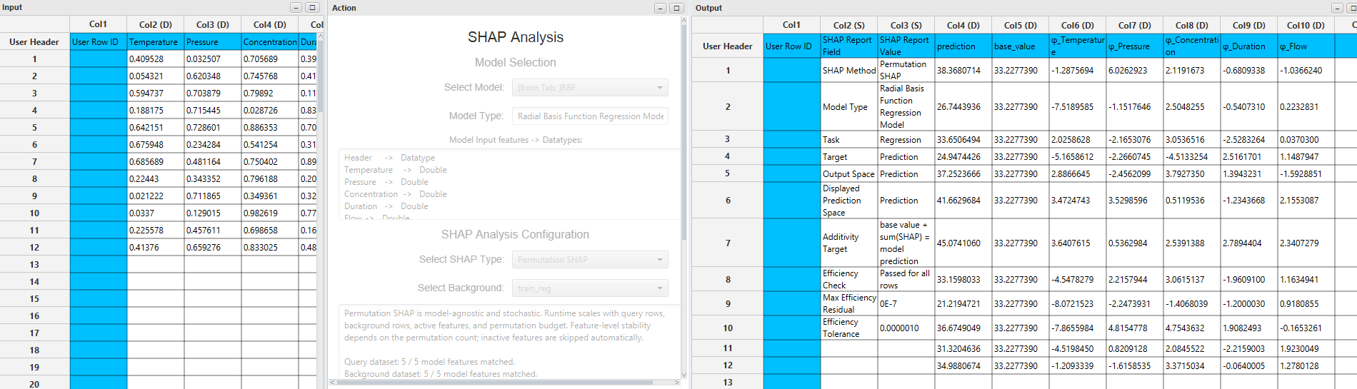
In this output, base_value is approximately 33.2277390 and the first query’s predicted response is 38.3680714. The feature contributions explain the increase from that baseline. Efficiency Check reports Passed for all rows. Although the reference dataset is shared with the Kernel example, the fitted RBF and kNN models differ, so their predictions and contributions need not match.
Inspect the baseline, explained prediction, efficiency result and feature contributions. Because Permutation SHAP is sampling-based, larger permutation counts generally improve stability; efficiency alone does not establish convergence. See Beeswarm Plot for the optional plot.
Linear SHAP
Linear SHAP is a model-specific method for supported linear models. Instead of evaluating many feature coalitions or sampled feature orderings, it uses the fitted coefficients of the linear model and the selected reference/background data to compute contributions relative to a baseline.2
In Isalos, Linear SHAP is the natural model-specific explanation path for supported Multiple Linear Regression (MLR) and Linear SGD regression models. These models already express the prediction as an additive sum of coefficient-weighted feature terms. Linear SHAP therefore does not need to approximate the model with a separate surrogate. It decomposes the fitted linear prediction directly.
Mathematical Formulation
For a linear regression model, the scalar prediction can be written as:
where \(\beta_0\) is the fitted intercept, \(\beta_j\) is the fitted coefficient for feature \(j\), and \(x_j\) is the query-row value for that feature. Isalos computes the reference value of each feature from the selected background data:
The Linear SHAP baseline is the model prediction at the background mean vector:
Each feature contribution is then the fitted coefficient multiplied by the feature’s deviation from its background mean:
This is not an approximation to the fitted linear model. Expanding the baseline plus the feature contributions gives:
The background means therefore provide the reference point, while the fitted coefficients determine the direction and size of each feature’s movement away from that reference point.
Background Interpretation
For Linear SHAP, the selected background dataset defines the reference feature means \(\mu_j\). The explanation therefore compares the query row to an average reference row, as seen by the fitted linear model. The baseline is not a generic constant chosen by the user; it is the fitted model evaluated at that background mean vector.
For example:
- If \(x_j > \mu_j\) and \(\beta_j > 0\), feature \(j\) contributes positively.
- If \(x_j > \mu_j\) and \(\beta_j < 0\), feature \(j\) contributes negatively.
- If \(x_j = \mu_j\), feature \(j\) contributes zero regardless of the coefficient.
The current Isalos Linear SHAP path is a mean-reference linear attribution path. It does not sample coalitions and does not estimate a covariance-aware conditional expectation model. This means the explanation is exact for the fitted linear equation under the selected mean-reference definition, but it does not attempt to redistribute effects caused by correlated features. If correlated predictors are present, the interpretation should be read as:
How does each feature’s difference from the selected background mean affect the linear prediction through its fitted coefficient?
Computational Technique in Isalos
For each query row, Isalos executes Linear SHAP as follows:
- Extract the fitted linear coefficients and intercept from the selected model adapter.
- Compute the mean of each model feature over the selected background rows.
- Compute the baseline as the model prediction at the background mean vector.
- Compute each feature contribution as coefficient multiplied by query-minus-background-mean.
- Return the exact reconstructed linear prediction and feature contributions.
- Verify that baseline plus feature contributions reconstructs the displayed linear prediction within numerical tolerance.
This is why Linear SHAP does not expose a coalition-sample or permutation-count field. Once the fitted coefficients and background means are known, the explanation is direct.
In vector form, the computation is:
where \(\beta\) is the fitted coefficient vector and \(\odot\) denotes elementwise multiplication. This direct formula is the computational technique: no coalition enumeration, feature permutation, or iterative numerical solve is required.
The dominant work is therefore small compared with model-agnostic methods. For \(N_{\mathrm{query}}\) explained rows, \(N_B\) background rows, and \(M\) model features, the background mean calculation scales as:
and the per-query contribution calculation scales as:
This is why Linear SHAP is typically much faster than Kernel SHAP or Permutation SHAP for supported linear models.
Using Linear SHAP in Isalos
Input
Linear SHAP requires a query datasheet and a background datasheet. The query datasheet contains the rows to be explained. The independently selected background datasheet defines the reference feature means \(\mu_j\) used in the exact linear contribution formula. Both datasets must contain the selected model’s input feature columns. Choose a representative background with compatible preprocessing, including when the fitted model has been imported.
Configuration
| Configuration field | Description |
|---|---|
| Select Model | Select a supported fitted linear model. The example below uses the model in the MLR tab, identified by the UI as Linear SGD regression. |
| Select SHAP Type | Confirm or choose Linear SHAP. For supported MLR and Linear SGD regression models, Isalos normally auto-selects this method. |
| Select Background | Select the reference dataset used to define the baseline feature means. Follow Choosing the Background Dataset, including for imported models. |
| Background Size (Rows) | Select the number of reference rows. |
| Beeswarm Plot | Generate a plot using the display selection described in Beeswarm Plot. |
| Select Features | Shown when Beeswarm Plot is ticked. Choose displayed features, or retain the default top ten. This does not limit the SHAP calculation. |
Output
The Linear SHAP output table contains the exact linear-model reconstruction for each query row. Each feature contribution is the fitted coefficient multiplied by the difference between the query value and the selected background mean for that feature. The reporting box’s Efficiency Check summarizes whether the baseline plus feature-level contributions reconstructs the displayed linear prediction within numerical tolerance.
Example
Input
This example explains the fitted linear regression model in the tab named MLR. The screenshot identifies its actual Model Type as Linear SGD Regression Model; a tab name alone does not determine the algorithm. The model is trained on the 100-row regression datasheet, which also supplies the Linear SHAP background. The separate 12-row regression test datasheet supplies the queries.
The regression training datasheet used as the background/reference data is shown below.
The regression test datasheet containing the query rows to be explained is shown below.
Configuration
Use Linear SHAP by selecting:
| Statistics \(\rightarrow\) SHAP Analysis \(\rightarrow\) Select SHAP Type: Linear SHAP |
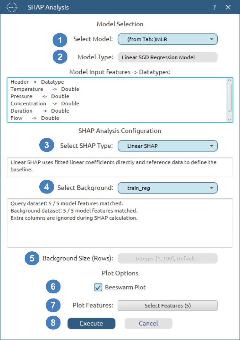
Select Modelchooses the fitted model in theMLRtab.Model TypedisplaysLinear SGD Regression Model. The feature panel below it lists the five model inputs and theirDoubledatatypes.- Confirm
Linear SHAP, the default for supported linear regression models. Select Backgroundis set totrain_reg.Background Size (Rows)is blank withDefault: -. Enter100to use all training reference rows. Linear SHAP then uses their feature means to define the reference prediction.Beeswarm Plotenables the optional plot described in Beeswarm Plot.Plot Features: Select Features (5)opens the feature selector. The screenshot selects all five features for display.- Click
Executeafter entering the background size.
The supplied screenshot numbers the lower controls from 3 to 8; the two unnumbered top fields correspond to steps 1 and 2 above. The message panel confirms that both query and background match all five fitted inputs. No sampling-budget field is needed for Linear SHAP.
Output
The output is a regression SHAP table with 12 explained rows. prediction contains the fitted linear prediction, base_value is the prediction at the background mean vector, and each feature-level SHAP column contains \(\beta_j(x_j-\mu_j)\) for that feature.
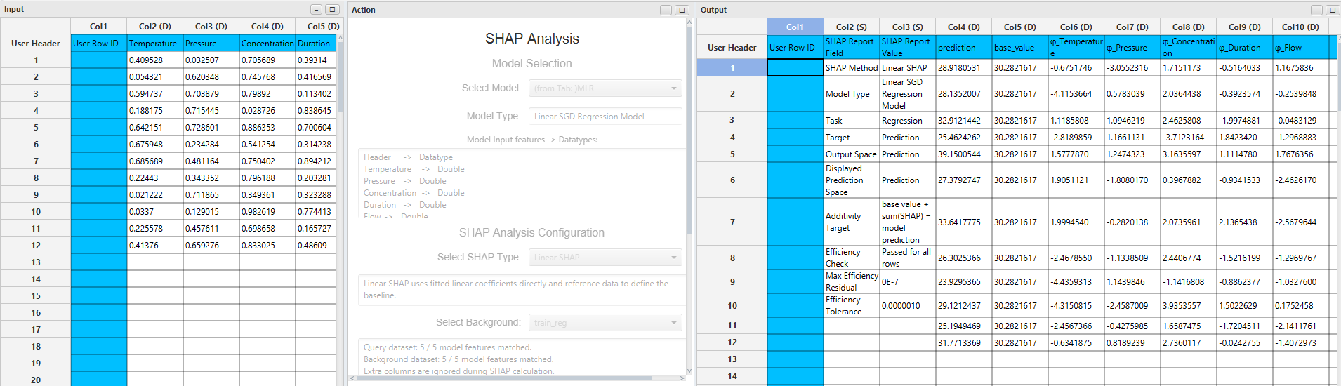
The reporting box confirms Linear SGD Regression Model. The baseline is approximately 30.2821617; for the first row, the contributions move the prediction down to 28.9180531. The global efficiency check passes for all rows. Each contribution’s sign depends on both the fitted coefficient and whether that row’s feature value is above or below its background mean.
Inspect the output table by checking that each contribution follows the fitted coefficient direction and that the baseline plus feature contributions exactly reconstructs the displayed linear prediction within numerical tolerance. If Beeswarm Plot was selected, inspect the generated plot after reviewing the table and interpret it using the shared Beeswarm Plot section.
Tree SHAP
Tree SHAP is a model-specific method for supported tree models. Rather than masking features by repeatedly constructing perturbed datasets, Tree SHAP uses the internal tree structure to compute feature contributions from the paths that observations follow through the fitted model.5
In Isalos, Tree SHAP uses the generic tree representation for supported decision-tree and forest models and native booster contributions for compatible XGBoost models. It explains their additive tree output directly. The reconstructed scalar must match the output space declared in the SHAP reporting box; it need not be the probability or transformed response displayed by an ordinary model-prediction node.
Mathematical Formulation
For tree ensembles, the model prediction can be written as a combination of tree outputs. A single decision tree has one tree output. Averaged ensembles, such as random forests, average multiple tree outputs. Boosted additive ensembles, such as compatible XGBoost regression models, sum multiple tree outputs with a model-specific base offset.
For a generic additive tree ensemble:
where \(c\) is a model-specific base offset and \(f_t(x)\) is the output of tree \(t\) for query row \(x\). For averaged ensembles, such as random forests, Isalos combines trees as:
For a boosted additive tree model, Isalos uses:
For a single tree, the query row follows one “hot” branch at each split. The opposite branch is the “cold” branch. Tree SHAP does not replace missing features by constructing a full hybrid row for every feature subset. Instead, it uses the training or reference mass reaching each tree node to define how path probability is split when a feature is unknown. At a split node \(u\) with hot child \(h\) and cold child \(c\), the path-dependent branch fractions are:
These fractions describe how much background or training mass would follow each branch when the split feature is unknown. The Tree SHAP recursion carries two quantities along each path:
- the zero fraction, describing how much path mass remains when the split feature is absent;
- the one fraction, describing how much path mass remains when the split feature is present.
For the split feature used at node \(u\), the present-feature path follows the hot branch selected by the query row. The absent-feature path distributes mass according to the node cover fractions. This is the tree-specific missing-feature philosophy: “missing” means that the tree path is averaged according to learned or reconstructed path mass, not that the feature value is set to zero or independently sampled for every coalition.
At each leaf, the leaf value is distributed across the features on the path using the Tree SHAP path weights. A compact way to describe the single-tree contribution is:
where \(\mathcal{L}_t\) is the set of leaves in tree \(t\), \(v_{\ell}\) is the value stored at leaf \(\ell\), and \(w_{j,\ell}\) is the Tree SHAP path weight assigned to feature \(j\) for that leaf. The path weight depends on the zero and one fractions accumulated along the path. Contributions are then summed across leaves and across trees.
For each tree represented by an Isalos adapter, the stored root expectation serves as the baseline and the reached leaf value serves as the prediction. The single-tree reconstruction is:
For additive boosted ensembles in raw output space, the final baseline and contributions are:
so that:
Here $F(x)$ denotes the raw additive tree output. It equals the displayed prediction only when the objective’s output transform is the identity.
Reference Interpretation
Tree SHAP uses tree structure and node cover counts to define the missing-feature behavior. The meaning of “missing” is therefore path-dependent: if a feature is not known, the recursion distributes mass between child branches according to cover fractions.
The role of reference data depends on the tree model:
- For tree models whose fitted structure already contains usable node cover information, the SHAP method can use that internal information directly.
- For Random Forest Tree SHAP in Isalos, reference rows may be requested to reconstruct path cover counts. These rows are not Kernel SHAP coalition background data; they are used to rebuild the branch-mass information needed by the tree recursion.
- XGBoost Tree SHAP uses the fitted booster’s stored statistics and native contribution calculation. It explains the raw output before any objective-specific probability or response transform. Isalos reports that space explicitly.
For the XGBoost classification example below, the UI path is the no-reference Tree SHAP path. The fitted booster supplies the path statistics and native contribution output, including its baseline. The query datasheet supplies the rows to be explained.
Computational Technique in Isalos
Isalos uses two execution paths for Tree SHAP. XGBoost models use the fitted booster’s native contribution calculation, described below. J48, Random Tree and Random Forest models use Isalos tree adapters and the shared recursion. Those adapters represent the fitted tree using:
- the split feature index;
- the split threshold;
- the branch direction rule;
- the node prediction value;
- the node cover count;
- the left and right child nodes.
The core Tree SHAP recursion then runs independently of the original model family. For each tree:
- Start at the root node.
- Determine which child is hot for the query row and which child is cold.
- Use child cover ratios to decide how absent-feature mass is split.
- Extend the path when a new split feature is encountered.
- Recurse down the hot branch with the feature-present fraction.
- Recurse down the cold branch with zero present-feature fraction for that split.
- Unwind the path if the same feature appears again lower in the tree, so repeated splits on the same feature remain one feature contribution.
- At each leaf, allocate the leaf value back to the features in the path using the path weights.
For an adapted single tree, the baseline is the stored root expectation and the prediction is the leaf value reached by the query row. For ensembles, Isalos aggregates single-tree SHAP values according to the model family:
| Tree family | Aggregation mode |
|---|---|
| Single decision tree | Single-tree output |
| Random forest | Average of tree outputs |
| Boosted trees | Sum of tree outputs plus base offset |
Tree SHAP distributes each tree’s contribution across the features used along its decision paths, then aggregates contributions across trees. This makes Tree SHAP especially suitable for supported tree-based models because it is aligned with the fitted model structure. It avoids repeatedly calling the model on hybrid datasets, and it avoids fitting a separate local surrogate.
For an ensemble whose trees are added, the final contribution is:
where \(a_t = 1\) for additive boosted trees and \(a_t = 1/T\) for averaged ensembles such as random forests. The computational cost scales with the number of trees and their path depths rather than with a user-selected coalition or permutation budget:
where \(T\) is the number of trees, \(L\) is the number of leaves considered by the recursion, and \(D\) is the maximum tree depth. This is why Tree SHAP does not show a coalition-sample or permutation-count field in the SHAP configuration window.
XGBoost Native Contributions and Output Space
For XGBoost classification and regression, Isalos requests feature contributions directly from the fitted booster. For each explained output, the returned values include one contribution per input feature and one baseline value. Their sum reconstructs the native raw margin. Isalos also checks the reconstruction against the model’s raw prediction before exporting the result.6
The model is already trained: this calculation explains its existing trees. The general Tree SHAP path interpretation still applies, but Isalos does not need to replay a separately parsed XGBoost tree ensemble to obtain these contributions.
Classification
For class $c$, let $F_c(x)$ be its raw margin, also called a class logit. The class-specific explanation satisfies:
The softmax transform converts all class margins into probabilities:
Here $K$ is the number of classes. A positive contribution raises the explained class’s margin relative to its baseline. It is not a probability-point contribution: the probability depends on the other class margins as well. Read the class identified by Target in the report box; the current SHAP configuration resolves this target internally rather than exposing a separate class-selection field.
Regression
For regression, write the displayed prediction as $\hat y(x)=h(F(x))$, where $h$ is the objective’s output transform. Native Tree SHAP reconstructs $F(x)$.
| XGBoost objective | Relationship to displayed prediction | SHAP scalar column |
|---|---|---|
reg:squarederror | $\hat y=F$ | prediction |
reg:gamma | $\hat y=\exp(F)$ | explained_regression_margin |
reg:tweedie | $\hat y=\exp(F)$ | explained_regression_margin |
For Gamma and Tweedie, feature contributions are on the log-response scale. Exponentiating individual SHAP values does not turn them into additive contributions in response units. To explain the ordinary predicted response instead, choose Kernel or Permutation SHAP and interpret its background-based explanation.
The corresponding output-space distinction applies to the Beeswarm plot: its SHAP coordinates use the units of the explained scalar reported in the table.
Using Tree SHAP in Isalos
Input
Tree SHAP requires a query datasheet containing the rows to be explained and the selected tree model’s input feature columns. For J48, Random Tree, and compatible XGBoost tree models, the Tree SHAP configuration may not require a background/reference selector because the needed tree-path information is already available through the fitted model or adapter. For supported Random Forest Tree SHAP cases, Isalos may request reference data to reconstruct path cover counts. When reference data is requested, use a representative compatible dataset as described in Choosing the Background Dataset.
Configuration
| Configuration field | Description |
|---|---|
| Select Model | Select a supported fitted tree model. For the example below, this is an XGBoost classification model. |
| Select SHAP Type | Confirm or choose Tree SHAP. For supported tree models, Isalos auto-selects this method when compatibility checks are satisfied. |
| Select Reference Data | Required for supported Random Forest Tree SHAP cases where reference rows are used to reconstruct path cover information. Not shown for all tree models. Follow Choosing the Background Dataset, including for imported models. |
| Reference Rows | Select the number of reference rows when reference data is required. |
| Beeswarm Plot | Generate a plot using the display selection described in Beeswarm Plot. |
| Select Features | Shown when Beeswarm Plot is ticked. Choose displayed features, or retain the default top ten. This does not limit the SHAP calculation. |
XGBoost Tree SHAP is available for supported tree boosters (gbtree and dart). The classification path supports multi:softprob and multi:softmax; regression includes squared-error, Gamma and Tweedie objectives. The reported output space depends on the objective. A linear booster is not a Tree SHAP model. Kernel or Permutation SHAP can instead explain a supported model’s ordinary prediction/probability output.
Output
The Tree SHAP output table contains the explained scalar, tree baseline, efficiency check, and one SHAP-value column for each model input feature. For Random Forest models, the explanation uses tree-path cover information reconstructed from the selected reference rows. For XGBoost, the native contributions reconstruct the raw additive output: the response for squared-error regression, a class margin for classification, or a regression margin for supported transformed objectives.
Example
Input
This example explains an XGBoost classification model trained on the 100-row classification datasheet with the five input features and the binary Class target. The separate 12-row classification test datasheet supplies the queries. This native XGBoost Tree SHAP path does not require a background selection: the fitted booster supplies the tree structure and training cover information used to compute its contributions.
The first rows of the classification training datasheet used to fit XGBoost are shown below.

The classification test datasheet containing the 12 query rows to be explained is shown below.

Configuration
Use Tree SHAP by selecting:
| Statistics \(\rightarrow\) SHAP Analysis \(\rightarrow\) Select SHAP Type: Tree SHAP |
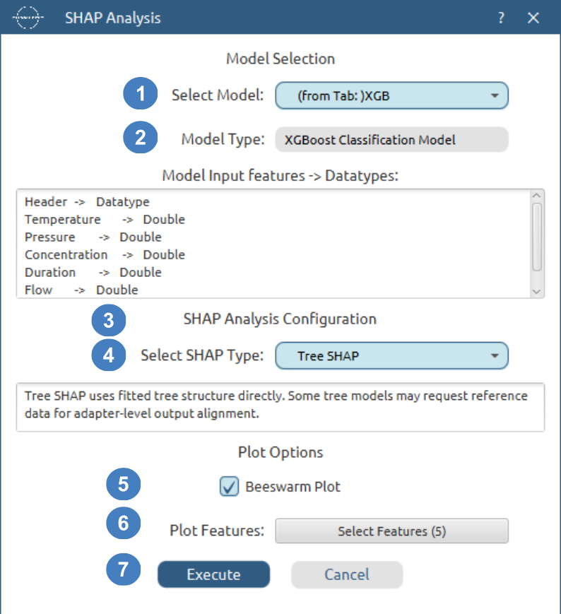
For the XGBoost classification example, the callouts identify the following:
Select Modelchooses the fitted model in theXGBtab.Model TypeconfirmsXGBoost Classification Model. The feature panel lists the fiveDoubleinputs.SHAP Analysis Configurationis the section heading, not an additional input. It separates the fitted-model information from the method selection below.Select SHAP TypeisTree SHAP, the default for this compatible fitted booster. The information panel explains that tree structure is used directly; this XGBoost path has no background-size or sampling-budget controls.Beeswarm Plotenables the optional plot. Its SHAP coordinates will use class-margin units, not probabilities.Plot Features: Select Features (5)opens the selector; all five features are selected for display.- Click
Executeto generate the explanations and the requested plot.
Output
The output contains one explanation per test row. The reporting box identifies the explained Target and raw class-margin Output Space. explained_class_margin contains the selected class’s raw score, base_value is the baseline in that same space, and the five feature contributions reconstruct the difference from the baseline. They are not additive probability changes; the conversion between margins and probabilities is explained in the XGBoost output-space subsection above.
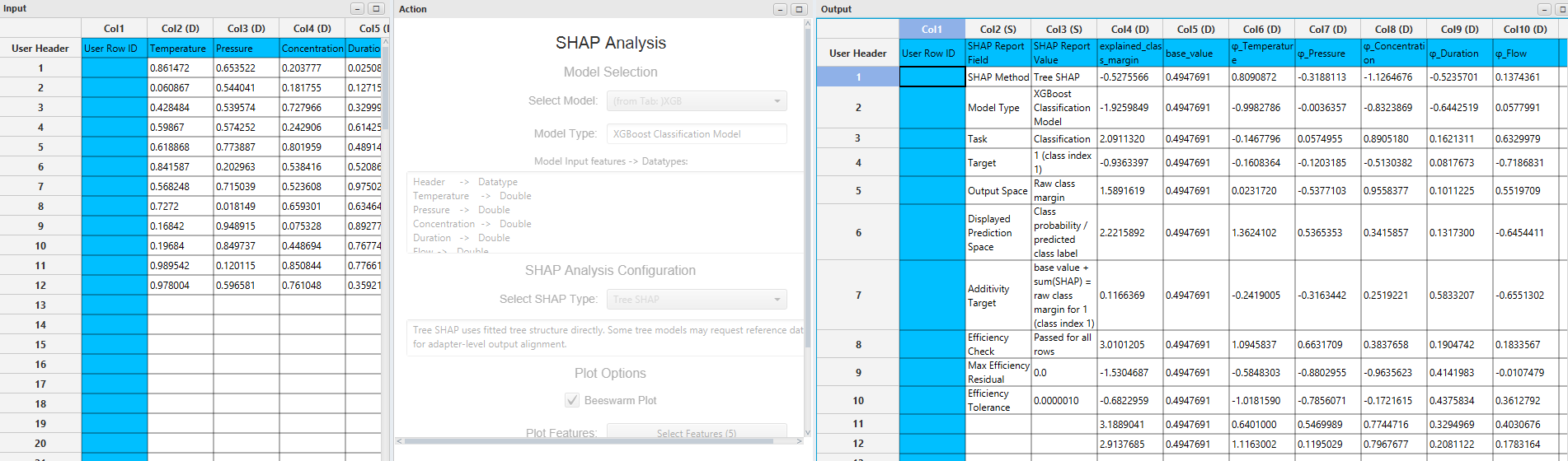
The screenshot identifies the target as 1 (class index 1) and the output space as Raw class margin. The baseline is approximately 0.4947691, while the first query’s explained margin is -0.5275566. A negative margin is valid: this column is not a probability. The separate Displayed Prediction Space report entry describes the model’s ordinary class-probability/predicted-label output, not the units of these SHAP values. The efficiency check passes for all rows in the reported margin space.
Check Efficiency Check and interpret any Beeswarm Plot in the same margin space. For squared-error regression, Tree SHAP instead explains the predicted response; Gamma and Tweedie use the reported regression-margin space.
Deep SHAP
Deep SHAP is a model-specific method for supported Multi-Layer Perceptron models. It uses the fitted neural network layers directly and propagates contribution multipliers backward through the network. The resulting feature attributions are averaged over background rows, which define the reference state of the model.2, 7
In Isalos, Deep SHAP is the default SHAP type for supported MLP models. The method is designed for dense affine neural-network layers with supported activation functions. It does not evaluate feature coalitions like Kernel SHAP and it does not sample reveal orderings like Permutation SHAP. Instead, it compares the neural-network activations of the query row against the activations of selected background rows, then propagates the resulting output difference back to the original input features.
Mathematical Formulation
Deep SHAP in Isalos is based on single-reference DeepLIFT-rescale attributions averaged over background rows. For one explained row \(x\) and one reference row \(r\), the method attributes the output difference:
to the original input features. For regression MLPs, \(f(\cdot)\) is the scalar model prediction. For classification MLPs, \(f(\cdot)\) is the selected class probability explained by the SHAP output table.
Averaging these single-reference attributions over the selected background rows gives:
and the baseline is:
For each reference row, the single-reference attributions satisfy:
Therefore the averaged explanation satisfies:
The central intuition is similar to DeepLIFT-style attribution. Instead of asking only for the local derivative of the prediction at the query row, Deep SHAP compares activations for the explained row against activations for background rows. This matters because a local derivative describes infinitesimal behavior at one point, while Deep SHAP attributes the finite movement from a reference activation state to the query activation state.
For a dense network layer, write the affine pre-activation and post-activation as:
where \(W^{(\ell)}\) and \(b^{(\ell)}\) are the fitted layer weights and biases, and \(g^{(\ell)}\) is the activation function for layer \(\ell\). For one query-reference pair, contribution propagation depends on activation differences:
where \(z_x\) is the activation input for the explained row and \(z_r\) is the activation input for a reference/background row. These differences are propagated backward to assign the final prediction difference to the original input features.
For deterministic elementwise activations, Isalos uses a rescale multiplier:
This multiplier is a finite-difference slope across the actual reference-to-query activation interval. For a linear activation it is exactly the ordinary derivative. For nonlinear activations, it captures the average effect of the activation over the interval between the reference pre-activation and the query pre-activation. When \(z_x\) and \(z_r\) are numerically indistinguishable, the finite-difference denominator is too small to use safely, so the implementation uses the activation derivative at the midpoint as a stable local fallback:
For an affine layer with weights \(W\), downstream multipliers are propagated backward through the weights:
The final input contribution for one reference row is:
The single-reference contributions reconstruct the difference between the query output and the reference output. Averaging across references then reconstructs the difference between the query output and the mean background output. This is the Deep SHAP equivalent of the baseline-to-prediction reconstruction used throughout the SHAP table.
Background Interpretation
The selected background rows define the reference neural-network states. For each background row, Isalos compares the query row against that reference row through every layer of the fitted MLP. The final SHAP value is the average of these reference-specific explanations.
This means that Deep SHAP explanations are sensitive to the chosen background distribution:
- A representative background set makes the baseline correspond to typical MLP behavior on relevant data.
- A very small background set can make explanations depend too strongly on a few reference activations.
- A background set from the wrong feature distribution can move hidden-layer reference activations into regions that are not meaningful for the selected model.
- Runtime scales directly with the number of background rows, so the background size is both an interpretability and performance choice.
Computational Technique in Isalos
Isalos converts the fitted MLP into a normalized dense-network representation containing the layer weights, biases, activation functions, and selected scalar output index. The Deep SHAP engine then executes the following process:
- Validate that the network is a supported dense affine MLP.
- Validate that the requested scalar output can be explained.
- Cache the forward-pass states for all selected background rows.
- Compute the baseline as the mean prediction over those background rows.
- For each query row, compute the query forward pass once.
- For each cached background pass, compare the query activations with the background activations layer by layer.
- Propagate contribution multipliers backward from the selected output through affine layers and supported activation functions.
- Multiply the input-level multipliers by \(x_i-r_i\) to obtain single-reference feature contributions.
- Average the contributions across all selected background rows.
- Verify that the averaged baseline plus feature contributions reconstructs the selected scalar output within numerical tolerance.
The background forward-pass cache is important computationally. It prevents Isalos from recomputing the same background activations for every query row. Each query still has to be compared against each background row, but the repeated background work is reused. This matters more as the number of background rows or the MLP depth increases.
Deep SHAP does not use a coalition or permutation sampling budget. Its runtime mainly scales with:
where \(N_{\mathrm{query}}\) is the number of explained rows, \(N_B\) is the number of background rows, and \(L\) represents the cost of propagating through the fitted MLP layers.
Final Softmax Handling
For MLP classification models with a final softmax output, Isalos explains one selected class probability. Softmax is multivariate:
Because the denominator couples all class logits, Isalos does not treat final softmax as independent elementwise activations. Instead, the final softmax probability is decomposed through exponentiation, summation, and division. For a query row \(x\) and reference row \(r\), define:
The explained class probability change is:
The division component is assigned by the exact two-input Shapley allocation over numerator and denominator changes:
The first bracket is the numerator contribution and the second bracket is the denominator contribution. This preserves the efficiency reconstruction of the explained class probability.
Hidden-layer softmax activations are not part of the first Deep SHAP UI support path. Final-output softmax is supported for selected-class probability explanations.
Using Deep SHAP in Isalos
Input
Deep SHAP requires a query datasheet and a background datasheet. The query datasheet contains the rows to be explained and must include the fitted MLP model’s input feature columns. The independently selected background datasheet defines the reference activations used by the Deep SHAP engine. The background rows should come from the same feature space and a representative data distribution for the selected MLP. Choose the reference population as described in Choosing the Background Dataset. For imported or pre-trained MLP models, upload a compatible background datasheet with the same preprocessing expected by the model.
Configuration
| Configuration field | Description |
|---|---|
| Select Model | Select a fitted Multi-Layer Perceptron model. The intended example for this section is an MLP classification model. |
| Select SHAP Type | Confirm or choose Deep SHAP. For supported MLP models, Isalos normally auto-selects this method. |
| Select Background | Select the reference dataset used to define background activations. Follow Choosing the Background Dataset, including for imported models. |
| Background Size (Rows) | Select the number of background rows. |
| Beeswarm Plot | Generate a plot using the display selection described in Beeswarm Plot. |
| Select Features | Shown when Beeswarm Plot is ticked. Choose displayed features, or retain the default top ten. This does not limit the SHAP calculation. |
Deep SHAP supports fitted MLP models through the implemented dense-layer path. For classification MLPs, the explained scalar is the selected class probability handled by the backend. Deep SHAP does not display coalition-sample or permutation-count controls because it averages layerwise attributions over background rows instead. The computational budget is therefore controlled mainly by the number of query rows, the number of selected background rows, and the size of the fitted MLP.
Output
The Deep SHAP output table contains the explained scalar MLP output, the mean background prediction, the efficiency check, and one SHAP-value column per model input feature. For MLP classification models, the explained scalar is the selected class probability handled by the backend.
Example
Input
This example explains a fitted MLP classification model trained in Isalos on the 100-row classification datasheet, with five input features and the binary Class target. The network architecture and training settings are configured in the model-training window, not in SHAP Analysis. Deep SHAP explains the selected fitted network without retraining it.
The same classification training datasheet, train_class, is selected as the background/reference source. The separate 12-row classification test datasheet supplies the queries.
The classification training datasheet used as the background/reference data is shown below.
The classification test datasheet containing the query rows to be explained is shown below.
Configuration
Use Deep SHAP by selecting:
| Statistics \(\rightarrow\) SHAP Analysis \(\rightarrow\) Select SHAP Type: Deep SHAP |
- Select the fitted MLP classification model.
- Confirm that
Model Typeidentifies the selected model as an MLP model. - Confirm or choose
Deep SHAP. For supported MLP models, this is the default SHAP type selected by Isalos. Select Backgroundis set totrain_class.Background Size (Rows)shows the valid range[1, 100]withDefault: -. Enter100to use all training rows as references; the placeholder shown is not an entered value.Beeswarm Plotenables the optional summary plot; see Beeswarm Plot.Plot Features: Select Features (5)opens the selector. Here all five inputs are selected for display; selection affects the plot, not the SHAP calculation.- Click
Executeafter entering the required background size.
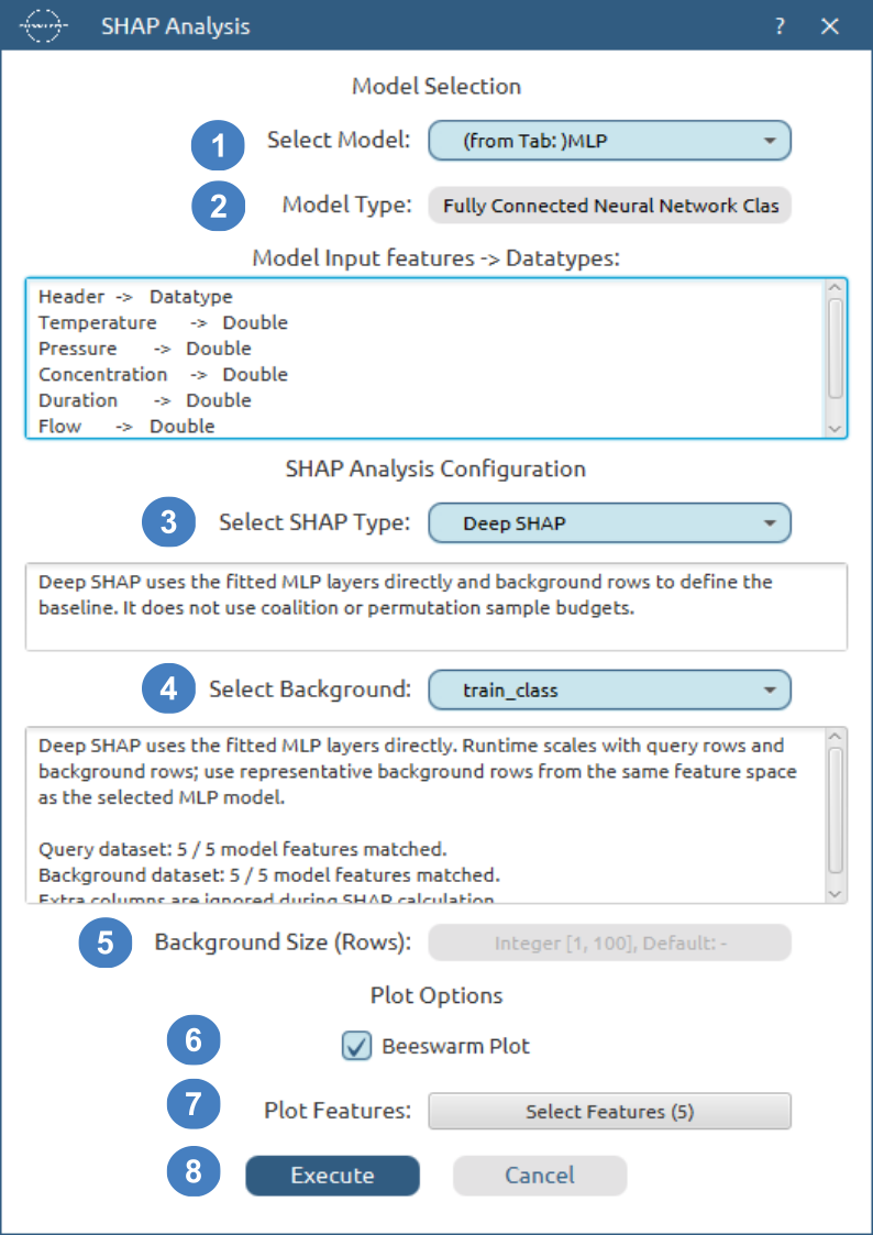
The Deep SHAP configuration window is intentionally shorter than the Kernel SHAP and Permutation SHAP windows. There is no coalition-sample or permutation-count field because Deep SHAP does not build explanations by sampling feature coalitions or feature orderings. Instead, the selected background rows are passed through the fitted MLP and used as reference activation states for layerwise contribution propagation.
Output
The output should be a classification SHAP table. Each row corresponds to one explained test row. The explained_class_probability column should contain the selected MLP class probability, base_value should contain the mean selected-class probability over the selected background rows, and each feature-level SHAP column should show how that feature moves the selected class probability away from the background baseline.
Inspect the mean background probability, the five feature contributions and the global efficiency result for the 12 queries. With the instructed background size of 100, base_value averages the selected class probability across all training reference rows. Read the reporting box’s Target rather than assuming which binary class is explained. Unlike the XGBoost classification example above, this Deep SHAP example explains probability, not a raw class margin.
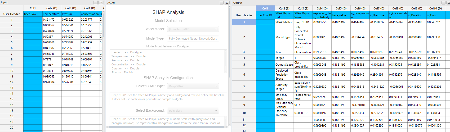
Here, the reporting box identifies Target as 1 and Output Space as Class probability. The baseline probability is approximately 0.4881492; the first query has an explained probability of 0.0913756. Its contributions therefore give a net decrease from the reference probability. The global efficiency check passes for all rows. Probabilities displayed as 1.0000000 are rounded table values and should not be interpreted as a guarantee of predictive certainty.
After reviewing the table, use the beeswarm plot to inspect how feature contributions vary across the explained test rows. The interpretation rules are shared across methods and are described in the Beeswarm Plot section.
How to Read SHAP Tables
The first two columns, SHAP Report Field and SHAP Report Value, form a reporting box. Each report field is written once. The remaining columns contain one explanation per query row, beginning with the explained scalar, then base_value, followed by one φ_... column per model input feature.
The reporting box and the explanation columns are independent parts of the table. A report entry beside an explanation does not describe only that query row. When fewer than ten query rows are explained, additional table rows can contain report entries with blank explanation cells.
Reporting Box
| Report field | Interpretation |
|---|---|
| SHAP Method | The method used for this result. |
| Model Type | The fitted model family being explained. |
| Task | Regression or classification. |
| Target | The response or class identified for this explanation. Check this before comparing classification results. |
| Output Space | The scalar space in which the baseline and SHAP values are expressed. |
| Displayed Prediction Space | The ordinary model-output space, which can differ from the explanation space. This entry describes the space; it is not an extra prediction column. |
| Additivity Target | The reconstruction relationship used for this output. This is the literal UI field name; the property checked here is efficiency/local reconstruction. |
| Efficiency Check | The reconstruction status across all explained rows. |
| Max Efficiency Residual | The largest absolute reconstruction discrepancy across the query rows. |
| Efficiency Tolerance | The numerical tolerance used for the check. |
Explanation Columns
| Output column | Description |
|---|---|
| prediction | The ordinary scalar model prediction being explained. |
| explained_class_probability | The probability of the class identified in the report box. |
| explained_class_margin | The selected XGBoost class’s raw margin before softmax. |
| explained_regression_margin | The raw XGBoost regression margin before the objective’s response transform. |
| base_value | The baseline in the same space as the explained scalar. |
| φ_feature | The contribution of that input feature, in the same output units. |
Only the scalar column appropriate to the selected method/model is included. For example, an XGBoost Gamma Tree SHAP table contains explained_regression_margin; it does not also include a response-scale prediction column.
For query row \(i\), let \(s_i\) denote the exported scalar. The residual is:
A small residual confirms that the exported contributions reconstruct the exported scalar. The current efficiency tolerance is \(10^{-6}\). The status is reported globally; there is no per-row efficiency_passed column. If the global check reports failures, the row residual can be calculated from the explanation columns to locate affected rows.
Efficiency alone does not prove that an approximate explanation is stable. For Kernel or Permutation SHAP, increase the sampling budget and compare results when sampling stability matters. Comparisons between implementations also require matching the fitted prediction function, query rows, background, explained class and output space.
Beeswarm Plot
A Beeswarm summarizes feature contributions across the query rows. Each point represents one row’s SHAP value for one feature. In the usual vertical-feature layout, the horizontal coordinate is the SHAP value and the categorical axis lists the features. Point colour represents the corresponding input feature value. The Feature Value label explains the colour scale; it is not a second numerical scale for the feature names.
Positive and negative coordinates increase or decrease the explained scalar relative to its baseline. Always read Target and Output Space in the SHAP table first: probability, raw-margin and response-scale explanations have different units.
Example Plot
The plot below is a separate display example with six descriptor features (D207, D484, D209, D488, D144, and D223). It illustrates a denser distribution of points than the 12-row method examples. It is not the output of the five-feature synthetic datasets above. The display controls apply across SHAP methods; obtain the target and scalar units from the reporting box for the particular run.
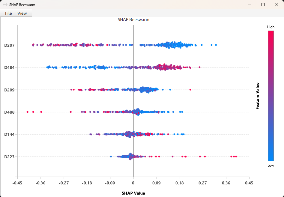
For D207, many high-value (pink) points lie on the negative side and many low-value (blue) points on the positive side: these observations contribute in opposite directions for the explained scalar. D484 shows a different pattern, with many high values on the positive side. These are patterns in the fitted model’s explanations, not evidence of causal effects. A dense cluster near zero indicates that many rows have small contributions for that feature.
Feature Ranking and Selection
Features are ranked by their mean absolute SHAP value over the explained rows:
This ranking measures the average magnitude of contributions for the chosen query population. It is not a causal effect or a measure of predictive accuracy.
Tick Beeswarm Plot in SHAP configuration to reveal Select Features. An unspecified selection displays the top ten features by \(I_j\), or all features if fewer than ten exist. The SHAP output table still contains every model feature. This initial display limit is useful for models with hundreds or thousands of inputs.
Inside the plot, Select Features opens the standard selection dialog. Add or remove features from the complete available list; the displayed subset is sorted by importance. Changing this display selection does not retrain the model or recompute its SHAP explanations. Save the project after making changes so that the selected plot can be restored with Show Chart when the project is reopened.
Colour and Point Placement
The default SHAP palette maps low feature values to blue and high feature values to pink. Colour bounds are calculated separately for each feature from the 5th and 95th percentiles of its values in the explained rows. Values outside these bounds use the endpoint colours. Colour therefore indicates relative values within a feature, not a common numerical scale across different features.
The colour values come from the query data supplied to SHAP, in its current preprocessing state. If those inputs are scaled, the colours represent scaled inputs. The palette does not display SHAP magnitude and does not indicate target labels.
Points with nearby SHAP values are stacked around the feature’s central line. The offset makes crowded regions visible without changing their numerical SHAP coordinate. The default point size is 7 and the point-spread setting is 25. Placement also takes the available feature spacing into account. Use a manageable feature selection and sufficient plot height when many rows are displayed.
Customization Controls
The customization panel is scrollable. The callouts in the following two screenshots group related controls, so each numbered section is described in full below. Numbers are read within their own screenshot: callout 4 in the upper panel identifies Colour Scale, whereas callout 4 in the lower panel identifies Axis Controls.
Upper Customization Panel
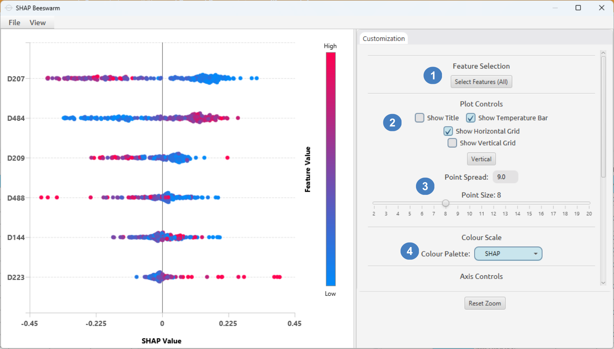
| Section number | Section / control | Explanation |
|---|---|---|
| 1 | Feature Selection — Select Features | Open the standard selector to add or remove displayed features from the complete available list. Select Features (All) is shown because all available features in this display example are included. Selection affects neither the fitted model nor the saved SHAP values. |
| 2 | Plot Controls — Show Title | Show or hide the plot title. It is unchecked here, so the title is absent from the chart, although the window title remains visible. |
| 2 | Show Temperature Bar | Show or hide the colour scale and its High/Low markers. It is enabled here. The bar describes feature values, not SHAP magnitudes. |
| 2 | Show Horizontal Grid / Show Vertical Grid | Toggle the two grid directions independently. Horizontal grid lines are enabled and vertical grid lines disabled in the screenshot. Vertical grid lines are also disabled by default for a new plot. |
| 2 | Orientation button | Switch the chart orientation using the button labelled Vertical in this capture. Read the displayed feature and numerical axes after changing orientation. |
| 3 | Point Spread | Control stacking distance around each feature’s central line. The screenshot uses 9.0, a customized value rather than the default 25. This changes point placement, not the SHAP coordinate. |
| 3 | Point Size | Change marker size with the slider. The screenshot uses 8; the default for a new SHAP plot is 7. Larger points can improve visibility but also increase crowding. |
| 4 | Colour Scale — Colour Palette | Select the colours used to encode the feature values. The SHAP palette shown maps low values to blue and high values to pink. Changing the palette does not change the data or contributions. |
Lower Customization Panel
Scroll down in the same panel to reach the remaining settings. Click either screenshot to view it at full size.
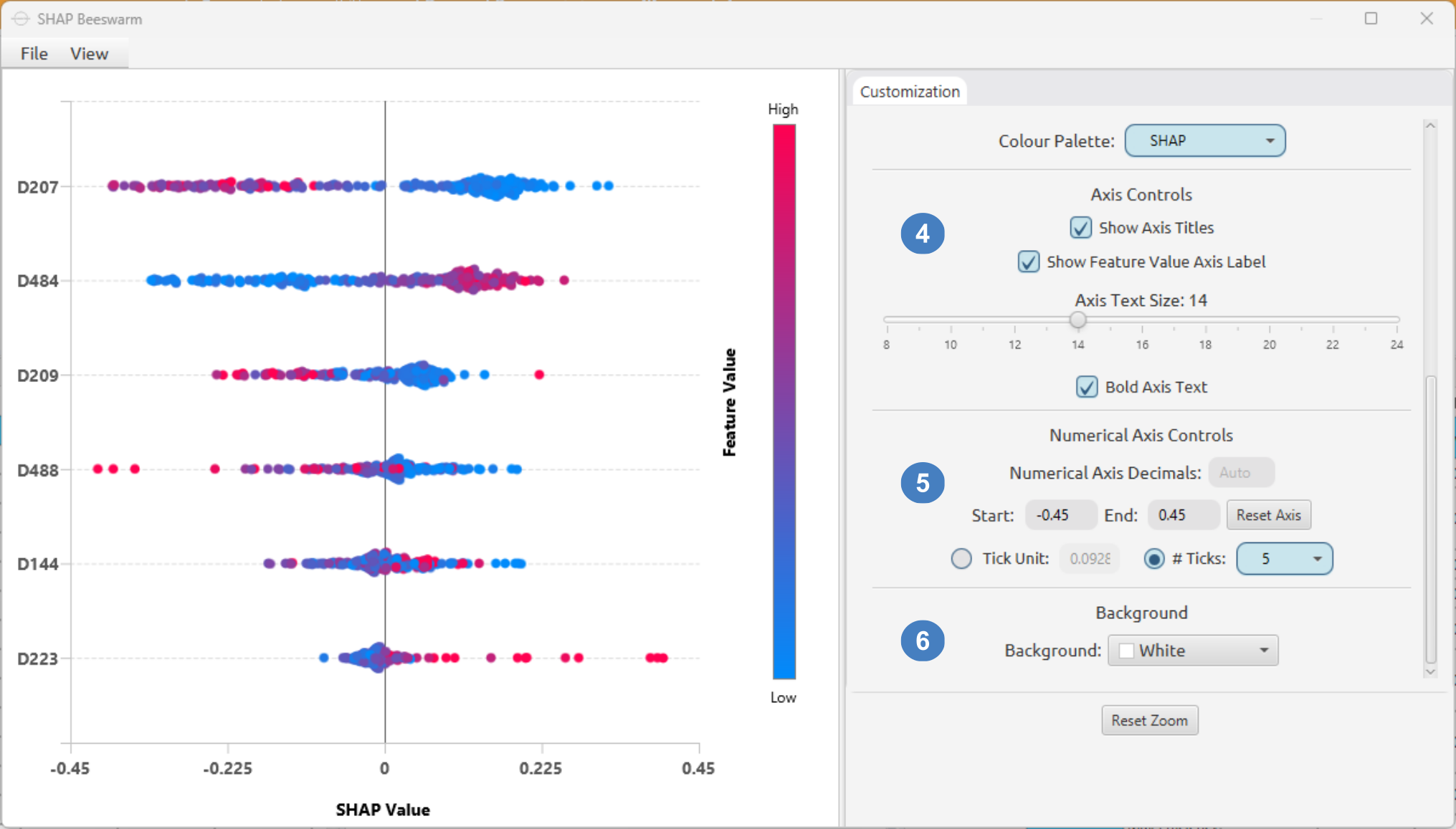
| Section number | Section / control | Explanation |
|---|---|---|
| 4 | Axis Controls — Show Axis Titles | Show or hide axis-title text. This is enabled in the screenshot. It controls titles rather than removing the feature names or numerical tick labels. |
| 4 | Show Feature Value Axis Label | Show or hide the Feature Value label independently of temperature-bar visibility, provided axis titles are enabled. It is enabled here. |
| 4 | Axis Text Size | Set axis-text size using the slider; 14 is selected here. The setting applies to feature labels, numerical ticks and the SHAP Value / Feature Value titles. |
| 4 | Bold Axis Text | Toggle bold axis text, including both axis titles. It is enabled in the screenshot. |
| 5 | Numerical Axis Controls — Numerical Axis Decimals | Leave blank for the Auto formatting shown, or enter 0–10 decimal places. This changes displayed tick labels, not the precision of stored SHAP values. |
| 5 | Start / End / Reset Axis | Set the displayed numerical range; the screenshot uses -0.45 to 0.45. Reset Axis restores the automatically determined range. A manually restricted range can hide points outside it without deleting them. |
| 5 | Tick Unit / # Ticks | Choose between numerical tick spacing and the tick-count control using the radio buttons. Here # Ticks is selected with 5; the inactive Tick Unit field is greyed out. |
| 6 | Background — Background | Choose the plot background colour. White is selected here. This is a visual setting and is unrelated to the SHAP reference/background dataset. |
| Unnumbered | Reset Zoom | Restore the unzoomed view. The button remains below the scrollable controls and is visible in the upper screenshot. |
These are display settings only. They do not require model retraining or another SHAP calculation. The screenshots deliberately include customized values; do not treat every value shown as an application default.
Interpreting Other SHAP Outputs
The method sections retain their configuration and output-table examples and refer here for plot interpretation. For any method, first inspect the table’s reporting box, then consider the direction and spread of contributions and the relative feature colours. A different feature selection changes only the displayed subset, while a different model, background or query population can change the underlying explanations. In particular, probability-space contributions and raw-margin contributions must not be interpreted as having the same units.
References
-
Shapley LS. A Value for n-Person Games. In: Kuhn HW, Tucker AW, editors. Contributions to the Theory of Games II. Princeton University Press; 1953:307-317. https://doi.org/10.1515/9781400829156-012
-
Lundberg SM, Lee SI. A Unified Approach to Interpreting Model Predictions. In: Advances in Neural Information Processing Systems 30; 2017. https://proceedings.neurips.cc/paper_files/paper/2017/hash/8a20a8621978632d76c43dfd28b67767-Abstract.html
-
SHAP documentation. shap.KernelExplainer API Reference. Accessed July 28, 2026. https://shap.readthedocs.io/en/stable/generated/shap.KernelExplainer.html
-
Strumbelj E, Kononenko I. Explaining prediction models and individual predictions with feature contributions. Knowledge and Information Systems. 2014;41:647-665. https://doi.org/10.1007/s10115-013-0679-x
-
Lundberg SM, Erion G, Chen H, DeGrave A, Prutkin JM, Nair B, Katz R, Himmelfarb J, Bansal N, Lee SI. From local explanations to global understanding with explainable AI for trees. Nature Machine Intelligence. 2020;2:56-67. https://doi.org/10.1038/s42256-019-0138-9
-
XGBoost documentation. Prediction and Learning Task Parameters. Accessed September 15, 2026. Prediction; Learning Task Parameters.
-
Shrikumar A, Greenside P, Kundaje A. Learning Important Features Through Propagating Activation Differences. In: Proceedings of the 34th International Conference on Machine Learning; PMLR 70:3145-3153; 2017. https://proceedings.mlr.press/v70/shrikumar17a
Version History
Introduced in Isalos Analytics Platform version to be confirmed.
Instructions last updated on September 2026